1. Introduction
Dispersion is the enhancement in flux of a diffusing substance in a non-uniform velocity field. This transport phenomenon is relevant in microfluidics, physiological flows, contaminant fate in the environment and analytical chemistry, for instance. The foundational work on dispersion is due to Taylor, who analysed the transport of a molecular solute in a steady Poiseuille flow (Taylor Reference Taylor1953). Diffusion acts to make the solute concentration uniform over the cross section of the tube at times long compared with  $a^2/\kappa$, where $a$ is the tube radius and $\kappa$ is the diffusivity of the solute. In addition, as solute diffuses it samples different flow streamlines, which enhances its longitudinal transport along the axis of the tube. Taylor showed that longitudinal variations in the cross-sectionally averaged solute concentration obey a diffusion equation in a frame of reference translating with the mean speed of the flow. The diffusion coefficient in this equation is not the solute diffusivity; rather, it is an effective diffusion coefficient, or dispersivity ($\kappa _{eff}$, say), equal to $a^2u_0^2/(192 \kappa )$, where ${{\frac {1}{2}}}u_0$ is the mean flow speed. This can be understood as follows: in a time $\tau =a^2/\kappa$ a solute molecule will experience a convective longitudinal displacement of order $u_0\tau =(u_0^2\tau )^{1/2}\tau ^{1/2}$, where $(u_0^2\tau )^{1/2}=a^2u_0^2/\kappa$ is the scaling for $\kappa _{eff}$. The factor of $1/192$ is particular to a tube of circular cross section. Consider a fixed amount of solute released into the flow at time $t=0$ at some location. At times $t\gg \tau$, Taylor's theory predicts that the centroid of the solute distribution moves with the mean speed of flow and that the solute spreads as a Gaussian about this centroid with variance proportional to $\kappa _{eff} t$. These predictions compare favourably against Taylor's own experiments on dispersion of potassium permanganate ($\mathrm {KMnO}_4$) solutions. Taylor's $\kappa _{eff}=a^2u_0^2/(192 \kappa )$ is valid if the Péclet number $Pe=u_0a/\kappa$, i.e. the ratio of diffusion $a^2/\kappa$ to advection $a/u_0$ times, is large. If this condition is not met, then longitudinal molecular diffusion cannot be neglected and the dispersivity is modified to $\kappa _{eff}=\kappa (1+{{\frac {1}{192}}}Pe^2)$. A plethora of variations on Taylor's theme have been considered; see Chu et al. (Reference Chu, Garoff, Przybycien, Tilton and Khair2019) for a review.
2. Overview
Ding (Reference Ding2023) (hereafter Reference DingD23) offers a fresh twist on dispersion. Specifically, Taylor considered dispersion of a solute that is electrically neutral. Reference DingD23 analysed the dispersion of an electrolyte solution; that is, when a pinch of salt is added to a non-uniform flow field. The salt dissociates into ions that diffuse and are advected by the flow, just as in Taylor's analysis. In addition, the ions would drift in an electric field since they are charged. However, how can an electric field arise if no voltage is externally applied? Well, electroneutrality of the solution must be obeyed at ionic separation distances beyond the Debye length. Consequently, the ionic charge density must sum to zero on such length scales, which constrains the ion concentrations to $\sum _{i=1}^nz_ic_i=0$, where $c_i$ and $z_i$ are the concentration and valence of the $\textit {i}$th species in an $n$-component electrolyte. The absence of an external voltage implies that the electrical current vanishes, which requires the additional constraint $\sum _{i=1}^nz_i\,\boldsymbol{j}_i=0$, where $\boldsymbol {j}_i=-\kappa _i\boldsymbol {\nabla } c_i-{{({\kappa _iz_ie}/{k_BT})}}c_i\boldsymbol {\nabla }\phi$ is the drift-diffusion flux of species $i$, in which $\kappa _i$ is the diffusion coefficient, $e$ is the charge on a proton, $k_B$ is Boltzmann's constant, $T$ is temperature and $\phi$ is the electric potential. Combining these two constraints shows that a spontaneous field $\boldsymbol {E}$ is induced, which equals
Chiang & Velegol (Reference Chiang and Velegol2014) claimed that (2.1) was first derived by Henderson (Reference Henderson1907). Equation (2.1) holds in the presence of a hydrodynamic velocity field $\boldsymbol {u}$, since the current owing to the flux of ions in this flow, $\sum _{i=1}^n\boldsymbol {u}z_ic_i$, is zero by electroneutrality. The spontaneous field exists only if the ions have unequal diffusion coefficients, which is practically always the case. For a binary electrolyte ($n=2$) we have $\boldsymbol {E}={{[({\kappa _1-\kappa _2})/({z_1\kappa _1-z_2\kappa _2})]}}\boldsymbol {\nabla } c_1$, where $z_2c_2+z_1c_1=0$ in an electroneutral solution. Physically, the field acts to speed up (slow down) the larger (smaller) ion of the pair in response to the diffusive flux arising from a concentration gradient. That is, the fluxes of the two ions are coupled by the requirement of electroneutrality. Mathematically, the coupled fluxes are $\boldsymbol {j}_i=-\kappa _{amb}\boldsymbol {\nabla } c_i$, where $\kappa _{amb}={{[{\kappa _1\kappa _2(z_1-z_2)}/({z_1\kappa _1-z_2\kappa _2})]}}$ is the ambipolar diffusion coefficient. Crucially, for a binary electrolyte the flux of species $i$ is proportional to the concentration gradient of that species only. Thus, in this case, Taylor's dispersion analysis holds; the only alteration needed is to replace the molecular diffusivity with the ambipolar diffusivity. Incidentally, this explains why Taylor's experiments on $\mathrm {KMnO_4}$, a binary electrolyte, can be properly compared to his theory that assumes a molecular, as opposed to ionic, solute.
The situation is essentially different for a multicomponent ($n>2$) electrolyte, an example of which would be two salts that share a common cation, such as in the pore-diffusion experiments of Gupta et al. (Reference Gupta, Shim, Issah, McKenzie and Stone2019) using sodium fluorescein and sodium chloride salts. The spontaneous field for a $n$-component electrolyte generates a coupled flux $\boldsymbol {j}_i=-\sum _{k=1}^n\mathcal {C}_{ik}\boldsymbol {\nabla } c_k$, in which
is the coupling coefficient relating the flux of species $i$ to a concentration gradient of species $k$ (Liu, Shang & Zachara Reference Liu, Shang and Zachara2019). Evidently, the flux of species $i$ is nonlinearly coupled to the concentrations of all ionic species for a multicomponent electrolyte. This leads to interesting diffusive dynamics even in the absence of a velocity field. Reference DingD23 analysed the even richer dynamics resulting from dispersive transport.
Reference DingD23 considered a multicomponent electrolyte in a channel with a longitudinally constant cross-section. The length of the channel is assumed to be much larger than its characteristic width. A unidirectional flow with velocity field $\boldsymbol {u}$, which could be steady or time-periodic, occurs in the channel. The concentration of the $i$th species satisfies the conservation equation
along with no flux conditions at the walls of the channel and prescribed initial distributions that are independent of the cross-sectional coordinates of the channel. Reference DingD23 utilised the electroneutrality and zero current constraints to recast (2.3) as
Equation (2.4) is equivalent to (2.3) in Reference DingD23; the nonlinear coupling of ionic fluxes is encapsulated in the off-diagonal terms of $\mathcal {C}_{ik}$. Reference DingD23 derived an equation for the longitudinal variation of the cross-sectionally averaged concentration of each ionic species, using a homogenisation procedure, which involved exploiting the small width-to-length ratio ($\epsilon$) of the channel, whereby ‘slow’ and ‘fast’ time scales on which ion diffusion occurs along the channel length and over the cross section, respectively, are introduced. Temporal variations in the flow are assumed to be on the slow time. Ion concentrations and electric potential are expanded as perturbation series in $\epsilon$, which are used with (2.4) to yield a hierarchy of problems. The main result in Reference DingD23 is the ‘effective equation’ (3.18), which describes the evolution of the concentration of ionic species at the slow time scale under a steady flow, in a reference frame moving with the mean flow speed. We rewrite (3.18) as
All variables in (2.5) are dimensionless: time $t$ is normalised on the diffusion time over the cross section; coordinate $x$ is normalised on a characteristic longitudinal distance; $\boldsymbol {c}$ is a vector containing concentrations of $n-1$ ionic species normalised by a reference concentration (the concentration of the $n$th ionic species can be found by electroneutrality); $F$ is a number that depends only on the form of the velocity field $\boldsymbol {u}$ (e.g. $F=1/192$ for steady flow in a tube); $Pe$ is a Péclet number as defined in § 1; and, finally, $\boldsymbol {D}$ is a ‘diffusion tensor’ whose elements are normalised by a reference diffusion coefficient and are closely related to the coupling coefficients $\mathcal {C}_{ik}$. The elements of $\boldsymbol {D}$ and its inverse, $\boldsymbol {D}^{-1}$, are defined in (3.9) and (3.12) of Reference DingD23.
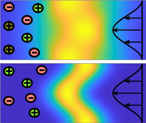
The diffusion tensor $\boldsymbol {D}$ degenerates to unity for a single species and reduces to a normalised ambipolar diffusion coefficient for a binary electrolyte. Taylor's analysis is thereby recovered in both cases. At $n=3$, however, $\boldsymbol {D}$ is a two-by-two matrix that depends nonlinearly on the concentrations of the ionic species. Reference DingD23 considered a three-ion system with $\kappa _1=1$, $\kappa _2=0.1$, $\kappa _3=1$, $z_1=1$, $z_2=1$ and $z_3=-2$ in a planar shear flow $\boldsymbol {u}=\cos (2{\rm \pi} y)\boldsymbol {e}_x$ (with zero mean) over the domain $-{\rm \pi} \leq x\leq 8{\rm \pi}$ and $0\leq y\leq 1$, where $\boldsymbol {e}_x$ is a unit vector in the flow direction. For this flow $F=(8{\rm \pi} ^2)^{-1}$. Figure 8 of Reference DingD23 plots ion concentration distributions at $t=0.2$ for $Pe=2$ obtained from numerical solution of (2.3) in Reference DingD23. Surprisingly, the concentration of the first ion species, $c_1$, bends opposite to the shear flow, which is due to the spontaneous field. At later times ($t=2$) the cross-sectionally averaged concentration profiles from the numerical solution compare well against the solution of the effective (3.18), which demonstrates the validity of the homogenisation scheme (figure 3 of Reference DingD23). Actually, the agreement is somewhat unexpected as $\epsilon =4$ in this case. The same system at $Pe=8$ was examined in figure 4 of Reference DingD23. Here, all ion distributions bend in the flow direction at early times ($t=0.2$) due to the stronger flow. Figure 6 computes the dispersivity vs $Pe$ for this three-ion system, where it is seen that: (i) the dispersivity can be a non-monotonic function of $Pe$ (unlike in Taylor's analysis); (ii) the ion with the largest dispersivity can change with $Pe$; and(iii) the dispersivity scales with $Pe^2$ at large $Pe$ (like in Taylor's analysis). A final point is that coupled fluxes can lead to non-Gaussian (even bimodal) ion distributions in the absence of flow (figure 7), although this effect diminishes in flow, e.g. at $Pe=2$ (figure 8).


 You have
Access
You have
Access
1. Introduction
Dispersion is the enhancement in flux of a diffusing substance in a non-uniform velocity field. This transport phenomenon is relevant in microfluidics, physiological flows, contaminant fate in the environment and analytical chemistry, for instance. The foundational work on dispersion is due to Taylor, who analysed the transport of a molecular solute in a steady Poiseuille flow (Taylor Reference Taylor1953). Diffusion acts to make the solute concentration uniform over the cross section of the tube at times long compared with $a^2/\kappa$, where $a$ is the tube radius and $\kappa$ is the diffusivity of the solute. In addition, as solute diffuses it samples different flow streamlines, which enhances its longitudinal transport along the axis of the tube. Taylor showed that longitudinal variations in the cross-sectionally averaged solute concentration obey a diffusion equation in a frame of reference translating with the mean speed of the flow. The diffusion coefficient in this equation is not the solute diffusivity; rather, it is an effective diffusion coefficient, or dispersivity ( $\kappa _{eff}$, say), equal to $a^2u_0^2/(192 \kappa )$, where ${{\frac {1}{2}}}u_0$ is the mean flow speed. This can be understood as follows: in a time $\tau =a^2/\kappa$ a solute molecule will experience a convective longitudinal displacement of order $u_0\tau =(u_0^2\tau )^{1/2}\tau ^{1/2}$, where $(u_0^2\tau )^{1/2}=a^2u_0^2/\kappa$ is the scaling for $\kappa _{eff}$. The factor of $1/192$ is particular to a tube of circular cross section. Consider a fixed amount of solute released into the flow at time $t=0$ at some location. At times $t\gg \tau$, Taylor's theory predicts that the centroid of the solute distribution moves with the mean speed of flow and that the solute spreads as a Gaussian about this centroid with variance proportional to $\kappa _{eff} t$. These predictions compare favourably against Taylor's own experiments on dispersion of potassium permanganate ( $\mathrm {KMnO}_4$) solutions. Taylor's $\kappa _{eff}=a^2u_0^2/(192 \kappa )$ is valid if the Péclet number $Pe=u_0a/\kappa$, i.e. the ratio of diffusion $a^2/\kappa$ to advection $a/u_0$ times, is large. If this condition is not met, then longitudinal molecular diffusion cannot be neglected and the dispersivity is modified to $\kappa _{eff}=\kappa (1+{{\frac {1}{192}}}Pe^2)$. A plethora of variations on Taylor's theme have been considered; see Chu et al. (Reference Chu, Garoff, Przybycien, Tilton and Khair2019) for a review.
2. Overview
Ding (Reference Ding2023) (hereafter Reference DingD23) offers a fresh twist on dispersion. Specifically, Taylor considered dispersion of a solute that is electrically neutral. Reference DingD23 analysed the dispersion of an electrolyte solution; that is, when a pinch of salt is added to a non-uniform flow field. The salt dissociates into ions that diffuse and are advected by the flow, just as in Taylor's analysis. In addition, the ions would drift in an electric field since they are charged. However, how can an electric field arise if no voltage is externally applied? Well, electroneutrality of the solution must be obeyed at ionic separation distances beyond the Debye length. Consequently, the ionic charge density must sum to zero on such length scales, which constrains the ion concentrations to $\sum _{i=1}^nz_ic_i=0$, where $c_i$ and $z_i$ are the concentration and valence of the $\textit {i}$th species in an $n$-component electrolyte. The absence of an external voltage implies that the electrical current vanishes, which requires the additional constraint $\sum _{i=1}^nz_i\,\boldsymbol{j}_i=0$, where $\boldsymbol {j}_i=-\kappa _i\boldsymbol {\nabla } c_i-{{({\kappa _iz_ie}/{k_BT})}}c_i\boldsymbol {\nabla }\phi$ is the drift-diffusion flux of species $i$, in which $\kappa _i$ is the diffusion coefficient, $e$ is the charge on a proton, $k_B$ is Boltzmann's constant, $T$ is temperature and $\phi$ is the electric potential. Combining these two constraints shows that a spontaneous field $\boldsymbol {E}$ is induced, which equals
Chiang & Velegol (Reference Chiang and Velegol2014) claimed that (2.1) was first derived by Henderson (Reference Henderson1907). Equation (2.1) holds in the presence of a hydrodynamic velocity field $\boldsymbol {u}$, since the current owing to the flux of ions in this flow, $\sum _{i=1}^n\boldsymbol {u}z_ic_i$, is zero by electroneutrality. The spontaneous field exists only if the ions have unequal diffusion coefficients, which is practically always the case. For a binary electrolyte ( $n=2$) we have $\boldsymbol {E}={{[({\kappa _1-\kappa _2})/({z_1\kappa _1-z_2\kappa _2})]}}\boldsymbol {\nabla } c_1$, where $z_2c_2+z_1c_1=0$ in an electroneutral solution. Physically, the field acts to speed up (slow down) the larger (smaller) ion of the pair in response to the diffusive flux arising from a concentration gradient. That is, the fluxes of the two ions are coupled by the requirement of electroneutrality. Mathematically, the coupled fluxes are $\boldsymbol {j}_i=-\kappa _{amb}\boldsymbol {\nabla } c_i$, where $\kappa _{amb}={{[{\kappa _1\kappa _2(z_1-z_2)}/({z_1\kappa _1-z_2\kappa _2})]}}$ is the ambipolar diffusion coefficient. Crucially, for a binary electrolyte the flux of species $i$ is proportional to the concentration gradient of that species only. Thus, in this case, Taylor's dispersion analysis holds; the only alteration needed is to replace the molecular diffusivity with the ambipolar diffusivity. Incidentally, this explains why Taylor's experiments on $\mathrm {KMnO_4}$, a binary electrolyte, can be properly compared to his theory that assumes a molecular, as opposed to ionic, solute.
The situation is essentially different for a multicomponent ( $n>2$) electrolyte, an example of which would be two salts that share a common cation, such as in the pore-diffusion experiments of Gupta et al. (Reference Gupta, Shim, Issah, McKenzie and Stone2019) using sodium fluorescein and sodium chloride salts. The spontaneous field for a $n$-component electrolyte generates a coupled flux $\boldsymbol {j}_i=-\sum _{k=1}^n\mathcal {C}_{ik}\boldsymbol {\nabla } c_k$, in which
is the coupling coefficient relating the flux of species $i$ to a concentration gradient of species $k$ (Liu, Shang & Zachara Reference Liu, Shang and Zachara2019). Evidently, the flux of species $i$ is nonlinearly coupled to the concentrations of all ionic species for a multicomponent electrolyte. This leads to interesting diffusive dynamics even in the absence of a velocity field. Reference DingD23 analysed the even richer dynamics resulting from dispersive transport.
Reference DingD23 considered a multicomponent electrolyte in a channel with a longitudinally constant cross-section. The length of the channel is assumed to be much larger than its characteristic width. A unidirectional flow with velocity field $\boldsymbol {u}$, which could be steady or time-periodic, occurs in the channel. The concentration of the $i$th species satisfies the conservation equation
along with no flux conditions at the walls of the channel and prescribed initial distributions that are independent of the cross-sectional coordinates of the channel. Reference DingD23 utilised the electroneutrality and zero current constraints to recast (2.3) as
Equation (2.4) is equivalent to (2.3) in Reference DingD23; the nonlinear coupling of ionic fluxes is encapsulated in the off-diagonal terms of $\mathcal {C}_{ik}$. Reference DingD23 derived an equation for the longitudinal variation of the cross-sectionally averaged concentration of each ionic species, using a homogenisation procedure, which involved exploiting the small width-to-length ratio ( $\epsilon$) of the channel, whereby ‘slow’ and ‘fast’ time scales on which ion diffusion occurs along the channel length and over the cross section, respectively, are introduced. Temporal variations in the flow are assumed to be on the slow time. Ion concentrations and electric potential are expanded as perturbation series in $\epsilon$, which are used with (2.4) to yield a hierarchy of problems. The main result in Reference DingD23 is the ‘effective equation’ (3.18), which describes the evolution of the concentration of ionic species at the slow time scale under a steady flow, in a reference frame moving with the mean flow speed. We rewrite (3.18) as
All variables in (2.5) are dimensionless: time $t$ is normalised on the diffusion time over the cross section; coordinate $x$ is normalised on a characteristic longitudinal distance; $\boldsymbol {c}$ is a vector containing concentrations of $n-1$ ionic species normalised by a reference concentration (the concentration of the $n$th ionic species can be found by electroneutrality); $F$ is a number that depends only on the form of the velocity field $\boldsymbol {u}$ (e.g. $F=1/192$ for steady flow in a tube); $Pe$ is a Péclet number as defined in § 1; and, finally, $\boldsymbol {D}$ is a ‘diffusion tensor’ whose elements are normalised by a reference diffusion coefficient and are closely related to the coupling coefficients $\mathcal {C}_{ik}$. The elements of $\boldsymbol {D}$ and its inverse, $\boldsymbol {D}^{-1}$, are defined in (3.9) and (3.12) of Reference DingD23.
The diffusion tensor $\boldsymbol {D}$ degenerates to unity for a single species and reduces to a normalised ambipolar diffusion coefficient for a binary electrolyte. Taylor's analysis is thereby recovered in both cases. At $n=3$, however, $\boldsymbol {D}$ is a two-by-two matrix that depends nonlinearly on the concentrations of the ionic species. Reference DingD23 considered a three-ion system with $\kappa _1=1$, $\kappa _2=0.1$, $\kappa _3=1$, $z_1=1$, $z_2=1$ and $z_3=-2$ in a planar shear flow $\boldsymbol {u}=\cos (2{\rm \pi} y)\boldsymbol {e}_x$ (with zero mean) over the domain $-{\rm \pi} \leq x\leq 8{\rm \pi}$ and $0\leq y\leq 1$, where $\boldsymbol {e}_x$ is a unit vector in the flow direction. For this flow $F=(8{\rm \pi} ^2)^{-1}$. Figure 8 of Reference DingD23 plots ion concentration distributions at $t=0.2$ for $Pe=2$ obtained from numerical solution of (2.3) in Reference DingD23. Surprisingly, the concentration of the first ion species, $c_1$, bends opposite to the shear flow, which is due to the spontaneous field. At later times ( $t=2$) the cross-sectionally averaged concentration profiles from the numerical solution compare well against the solution of the effective (3.18), which demonstrates the validity of the homogenisation scheme (figure 3 of Reference DingD23). Actually, the agreement is somewhat unexpected as $\epsilon =4$ in this case. The same system at $Pe=8$ was examined in figure 4 of Reference DingD23. Here, all ion distributions bend in the flow direction at early times ( $t=0.2$) due to the stronger flow. Figure 6 computes the dispersivity vs $Pe$ for this three-ion system, where it is seen that: (i) the dispersivity can be a non-monotonic function of $Pe$ (unlike in Taylor's analysis); (ii) the ion with the largest dispersivity can change with $Pe$; and(iii) the dispersivity scales with $Pe^2$ at large $Pe$ (like in Taylor's analysis). A final point is that coupled fluxes can lead to non-Gaussian (even bimodal) ion distributions in the absence of flow (figure 7), although this effect diminishes in flow, e.g. at $Pe=2$ (figure 8).
3. Outlook
Reference DingD23 has shown that coupled ionic fluxes fundamentally affect dispersion of multicomponent electrolytes. The dispersive transport is richer than for an uncharged solute, due to the inherent nonlinearity introduced by this coupling. Extensions to Reference DingD23 can readily be envisioned. For instance, the generalisation of (3.18) in Reference DingD23 to curved channels or straight channels with longitudinal variations in cross-sectional area or longitudinal slip-stick patterning. Electrolytes with $n>3$ components, some of which may not completely dissociate, would also be interesting to consider, in steady and unsteady flows. One should also analyse the evolution of ionic concentrations in unbounded flows, such as simple shear, or flows with closed streamlines. Practical applications to the measurement of relative amounts of species in a multicomponent ionic solution were suggested by Reference DingD23. The interesting work of Reference DingD23 provides a foundation for these future studies.
Declaration of interests
The authors report no conflict of interest.