


1 Introduction
We are interested in the distribution of directions of saddle connections on translation surfaces. A translation surface is a pair
 $(X,\omega )$
, where X is a compact, connected Riemann surface of genus g and
$(X,\omega )$
, where X is a compact, connected Riemann surface of genus g and
 $\omega $
is a non-zero holomorphic 1-form on X. The singular flat metric induced by
$\omega $
is a non-zero holomorphic 1-form on X. The singular flat metric induced by
 $\omega $
has isolated singularities at the zeros of
$\omega $
has isolated singularities at the zeros of
 $\omega $
, with a zero of order k corresponding to a point with cone angle
$\omega $
, with a zero of order k corresponding to a point with cone angle
 $2\pi (k+1)$
.
$2\pi (k+1)$
.
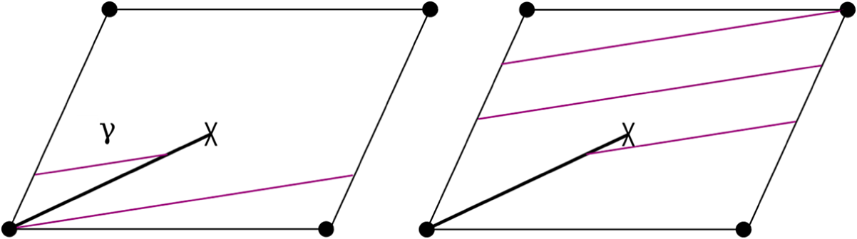
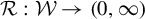
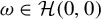
A saddle connection is a geodesic segment in the flat metric connecting two (not necessarily distinct) singular points, with no singular points in its interior. See Figure 1 for an example of a saddle connection on a translation surface. Integrating
 $\omega $
over
$\omega $
over
 $\gamma $
yields the holonomy vector of
$\gamma $
yields the holonomy vector of
 $\gamma $
, which keeps track of how far and in what direction
$\gamma $
, which keeps track of how far and in what direction
 $\gamma $
travels. We write
$\gamma $
travels. We write
 $$ \begin{align*}v_\gamma := \int_\gamma \omega \in {\mathbb{C}}.\end{align*} $$
The set of all holonomy vectors,
 $$ \begin{align*}\Lambda_\omega = \{v_\gamma: \gamma \text{ is an oriented saddle connection on } (X,\omega)\}\subset {\mathbb{C}}\end{align*} $$
is a discrete subset of the plane, see e.g. [Reference Hubert and Schmidt16].
A saddle connection
 $\gamma $
on a translation surface. This translation surface is an example of a doubled slit torus.
$\gamma $
on a translation surface. This translation surface is an example of a doubled slit torus.
The counting and distribution of saddle connections and their holonomy vectors is a very well-studied problem and we review the relevant history in §1.1. Our motivating question is understanding how random the set of saddle connection directions are for some classes of translation surfaces. We study this by considering the gap distribution of slopes of holonomy vectors which we now describe.
The slopes of saddle connections of a translation surface
 $(X,\omega )$
in the first quadrant and underneath the diagonal are given by
$(X,\omega )$
in the first quadrant and underneath the diagonal are given by
 $$ \begin{align*}\mathcal S(\Lambda_{\omega}) := \bigg\{\text{slope}(w) = \frac{w_2}{w_1} \,\bigg |\, w =w_1+i w_2\in \Lambda_{\omega},0<w_1,0\le w_2\le w_1\bigg\}.\end{align*} $$
We will see in §2.2 why we need the restriction to the first quadrant and underneath the first diagonal. In fact, by applying a rotation matrix, we can move saddle connections outside of the first quadrant and underneath the diagonal into it so that this restriction is a mild one.
Let
 $\mathcal S^R(\Lambda _{\omega }) $
be the set of slopes of saddle connections in
$\mathcal S^R(\Lambda _{\omega }) $
be the set of slopes of saddle connections in
 $\omega $
that are in the first quadrant, underneath the diagonal, and in the ball of radius R about 0 with respect to the max norm on
$\omega $
that are in the first quadrant, underneath the diagonal, and in the ball of radius R about 0 with respect to the max norm on
 ${\mathbb {R}}^2$
,
${\mathbb {R}}^2$
,
 $$ \begin{align*}\mathcal S^R(\Lambda_{\omega}) = \bigg\{\text{slope}(w) = \frac{w_2}{w_1} \,\bigg |\, w \in \Lambda_{\omega}, w_1\in (0,R], w_2\in[0,w_1] \bigg\}. \end{align*} $$
Let
 $N(\omega , R):= |\mathcal S^R(\Lambda _{\omega })|$
and write the elements of
$N(\omega , R):= |\mathcal S^R(\Lambda _{\omega })|$
and write the elements of
 $\mathcal S^R(\Lambda _\omega )$
in increasing order:
$\mathcal S^R(\Lambda _\omega )$
in increasing order:
 $$ \begin{align*}\mathcal S^R(\Lambda_{\omega}) = \{s_0 = 0<s_1<\cdots <s_{N(\omega, R)} \}. \end{align*} $$
By the seminal work of Eskin and Masur [Reference Eskin and Masur13], for almost every translation surface, there are positive constants
 $ c_1 = c_1(\omega ) \le c_2 = c_2(\omega )$
so that
$ c_1 = c_1(\omega ) \le c_2 = c_2(\omega )$
so that
 $$ \begin{align*}c_1 R^2 \le N(\omega, R) \le c_2 R^2.\end{align*} $$
Later on, Eskin, Marklof, and Morris [Reference Eskin, Marklof and Morris12] obtained similar asymptotics for branched covers of lattice surfaces.
We are interested in slope gaps and since
 $N(\omega , R)$
grows quadratically, then it is natural to consider the set of renormalized slope gaps,
$N(\omega , R)$
grows quadratically, then it is natural to consider the set of renormalized slope gaps,
 $$ \begin{align} \mathcal G^R(\Lambda_{\omega}) = \{R^2\cdot(s_i-s_{i-1})\mid i = 1,\ldots, N(\omega, R)\}. \end{align} $$
The gap distribution of saddle connection directions on a translation surface
 $(X,\omega )$
is given by the weak-* limit as
$(X,\omega )$
is given by the weak-* limit as
 $R \rightarrow \infty $
of the probability measures
$R \rightarrow \infty $
of the probability measures
 $$ \begin{align} \eta_R(\omega) = \frac{1}{N(\omega, R)} \sum_{x \in \mathcal G^R(\Lambda_{\omega})} \delta_x \end{align} $$
if it exists.
Evaluating the weak-* limit of these measures on the indicator function of an interval I, we obtain
 $$ \begin{align} \lim_{R\to\infty}\frac{| \mathcal G^R(\Lambda_{\omega}) \cap I|}{N(\omega, R)} \end{align} $$
the proportion of gaps in an interval I.
1.1 Motivations for gap distributions
The counting and distribution properties of saddle connections and their directions have been studied extensively. Masur [Reference Masur18] showed the angles of saddle connections are dense on the circle for any translation surface. Vorobets [Reference Vorobets30] and Eskin and Masur [Reference Eskin and Masur13] showed that the angles equidistribute on the circle for a generic translation surface. More recently, Dozier [Reference Dozier9, Theorem 1.3] showed that for every translation surface, the distribution of angles converge to a measure that is in the same measure class as the Lebesgue measure on the circle. Precise descriptions of their results are in the references above, but they suggest that angles (and thus slopes) seem to behave ‘randomly’ at first glance. Thus, the gap distribution of translation surfaces can be thought of as a second test of randomness that yields insight to the fine-scale statistics of holonomy vectors.
Probability theory provides some context for what one would expect from ‘truly random’ gaps. In the case of a sequence of independent identically distributed uniform random variables on
 $[0, 1]$
, the gaps converge to an exponential distribution. Following [Reference Athreya2], we call gap distributions that deviate from an exponential distribution exotic.
$[0, 1]$
, the gaps converge to an exponential distribution. Following [Reference Athreya2], we call gap distributions that deviate from an exponential distribution exotic.
1.2 Main results
We compute the gap distribution for the set of translation surfaces that arise from gluing two identical tori along a slit. See Figure 1. We call such a surface a doubled slit torus. Every doubled slit torus has genus two and two cone-type singularities of angle
 $4\pi $
. Denote the class of doubled slit tori by
$4\pi $
. Denote the class of doubled slit tori by
 ${\mathcal {E}}.$
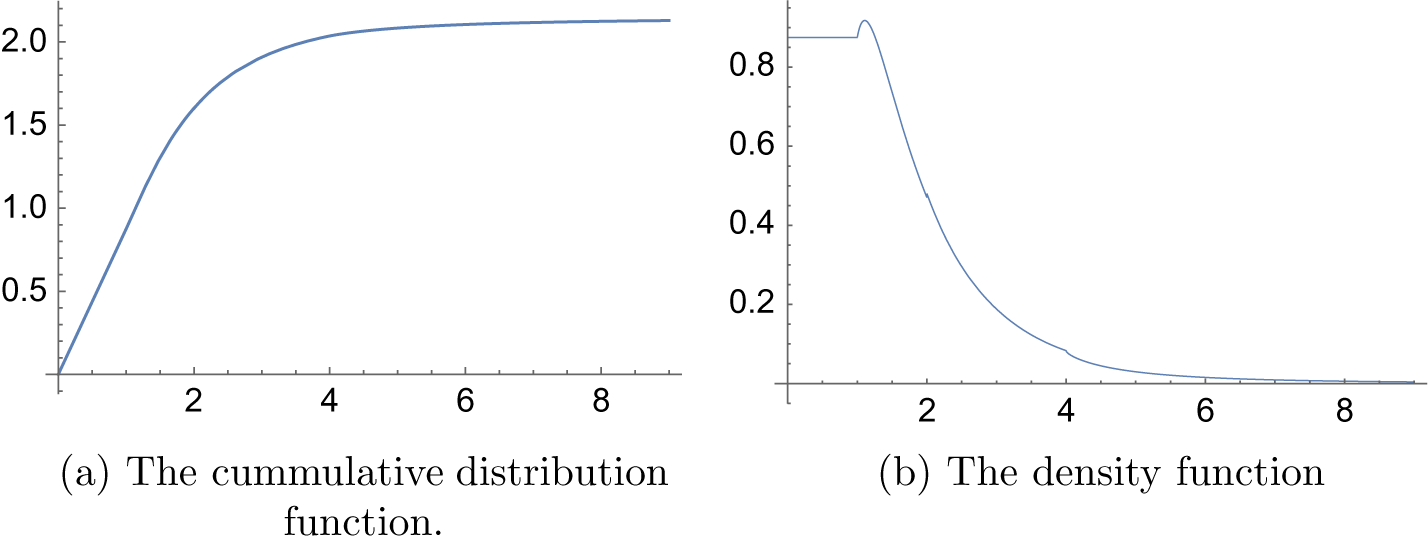
We prove that the gap distribution of doubled slit tori exists and is given by an explicit density function. This provides the first explicit computation of a gap distribution for a non-lattice surface.
${\mathcal {E}}.$
We prove that the gap distribution of doubled slit tori exists and is given by an explicit density function. This provides the first explicit computation of a gap distribution for a non-lattice surface.
Theorem 1.1. There is a limiting probability density function
 $ f : [0,\infty ) \to [0,\infty )$
, with
$ f : [0,\infty ) \to [0,\infty )$
, with
 $$ \begin{align*}\lim_{R\to\infty}\frac{| \mathcal G^R (\Lambda_\omega) \cap I|}{N(\omega, R)}=\int_I f(x)\,dx\end{align*} $$
for almost every doubled slit torus
 $\omega $
with respect to an
$\omega $
with respect to an
 ${\textrm {SL}}_2({\mathbb {R}})$
-invariant probability measure on
${\textrm {SL}}_2({\mathbb {R}})$
-invariant probability measure on
 ${\mathcal {E}}$
that is in the same measure class as the Lebesgue measure.
${\mathcal {E}}$
that is in the same measure class as the Lebesgue measure.
The density function is continuous, piecewise differentiable with four points of non-differentiability, and each piece is expressed in terms of elementary functions.
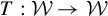
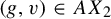
Proportion of gaps for doubled slit tori.
The proof of Theorem 1.1 can be found in §4 and an explicit description of the cumulative distribution function can be found in Appendix A.1.3. As a corollary, we also show that the gap distribution has a quadratic tail so that the gap distribution of doubled slit tori is exotic (Theorem 4.4(3)). We prove other results related to the gap distribution, but we wait until §4 Theorem 4.4 before more precisely stating them.
Perhaps surprisingly, Theorem 1.1 will follow from the following dynamical result (relevant definitions will be given in §2).
Theorem 1.2. The set
 ${\mathcal {W}}$
consisting of doubled slit tori with a horizontal saddle connection of length less than or equal to
${\mathcal {W}}$
consisting of doubled slit tori with a horizontal saddle connection of length less than or equal to
 $1$
forms a transversal for the space of doubled slit tori
$1$
forms a transversal for the space of doubled slit tori
 ${\mathcal {E}}$
under horocycle flow. There is a four-dimensional parameterization of
${\mathcal {E}}$
under horocycle flow. There is a four-dimensional parameterization of
 ${\mathcal {W}}$
(see Proposition 3.10) and the return time map in these coordinates is given explicitly (see Theorem 3.11).
${\mathcal {W}}$
(see Proposition 3.10) and the return time map in these coordinates is given explicitly (see Theorem 3.11).
In fact, the connection between the slope gap questions and return times on moduli space is relatively well understood, see Athreya [Reference Athreya2] or §2.3 where we recall this connection. The main contribution of this theorem is the explicit return time map (Theorem 3.11) that requires new techniques arising from the high dimensionality of the parameter space. Another key ingredient in proving Theorem 1.2 is the study of unipotent flows on the space of affine lattices. By an affine lattice we simply mean a set of the form
 $g{\mathbb {Z}}^2+v$
, where
$g{\mathbb {Z}}^2+v$
, where
 $g\in {\textrm {SL}}_2({\mathbb {R}})$
and
$g\in {\textrm {SL}}_2({\mathbb {R}})$
and
 $v\in {\mathbb {R}}^2$
. We prove the following result for the space of affine lattices.
$v\in {\mathbb {R}}^2$
. We prove the following result for the space of affine lattices.
Theorem 1.3. The set
 $\Omega $
consisting of affine lattices with a horizontal vector of length less than or equal to
$\Omega $
consisting of affine lattices with a horizontal vector of length less than or equal to
 $1$
forms a transversal for the space of affine lattices
$1$
forms a transversal for the space of affine lattices
 $AX_2$
under horocycle flow. There is a four-dimensional parameterization of
$AX_2$
under horocycle flow. There is a four-dimensional parameterization of
 $\Omega $
(see Proposition 3.5) and the return time map in these coordinates is given explicitly (see Theorem 3.6).
$\Omega $
(see Proposition 3.5) and the return time map in these coordinates is given explicitly (see Theorem 3.6).
In addition to using the above theorem to prove Theorem 1.2, we also use it to prove a slope gap question for affine lattices that we phrase in §2.5.
1.3 Why doubled slit tori are important
The space
 ${\mathcal {E}}$
of doubled slit tori has a long history of being studied to provide insight into general questions on the dynamics and geometry of translation surfaces. That the space and the surfaces within it have very concrete descriptions make it an excellent testing ground for conjectures.
${\mathcal {E}}$
of doubled slit tori has a long history of being studied to provide insight into general questions on the dynamics and geometry of translation surfaces. That the space and the surfaces within it have very concrete descriptions make it an excellent testing ground for conjectures.
For example, Masur [Reference Masur and Tabachnikov.20] showed that the space
 ${\mathcal {E}}$
provided the first examples of higher genus surfaces with a minimal but non-uniquely ergodic directional flow. Cheung [Reference Cheung6] used these surfaces to show that an upper bound on Hausdorff dimension of the directions which are non-ergodic was sharp. A dichotomy on the Hausdorff dimension of such directions for doubled slit tori was later given by Cheung et al [Reference Cheung, Hubert and Masur7].
${\mathcal {E}}$
provided the first examples of higher genus surfaces with a minimal but non-uniquely ergodic directional flow. Cheung [Reference Cheung6] used these surfaces to show that an upper bound on Hausdorff dimension of the directions which are non-ergodic was sharp. A dichotomy on the Hausdorff dimension of such directions for doubled slit tori was later given by Cheung et al [Reference Cheung, Hubert and Masur7].
The space
 ${\mathcal {E}}$
is also interesting from the point of view of the
${\mathcal {E}}$
is also interesting from the point of view of the
 ${\textrm {SL}}_2({\mathbb {R}})$
action on translation surfaces. In the remarkable paper [Reference McMullen21], McMullen completely classifies orbit closures (under
${\textrm {SL}}_2({\mathbb {R}})$
action on translation surfaces. In the remarkable paper [Reference McMullen21], McMullen completely classifies orbit closures (under
 ${\textrm {SL}}_2({\mathbb {R}})$
) of genus 2 translation surfaces. One consequence of his work is that there are translation surfaces that have non-closed
${\textrm {SL}}_2({\mathbb {R}})$
) of genus 2 translation surfaces. One consequence of his work is that there are translation surfaces that have non-closed
 ${\textrm {SL}}_2({\mathbb {R}})$
orbits but are not dense. These intermediate orbit closures consist of an infinite family called the eigenform loci. The space
${\textrm {SL}}_2({\mathbb {R}})$
orbits but are not dense. These intermediate orbit closures consist of an infinite family called the eigenform loci. The space
 ${\mathcal {E}}$
is a part of this family and often called the Eigenform locus of discriminant four in the literature.
${\mathcal {E}}$
is a part of this family and often called the Eigenform locus of discriminant four in the literature.
1.4 Some history of gap distributions
This paper makes use of unipotent flows on the space of affine lattices to prove a gap distribution result for doubled slit tori. Elkies and McMullen [Reference Elkies and McMullen10] famously used unipotent flows on the space of affine lattices to compute the distribution of gaps of the sequence
 $(\sqrt {n})_{n\in {\mathbb {N}}}$
on the unit circle. Similarly, Marklof and Strömbergsson [Reference Marklof and Strömbergsson17] used dynamics on the space of affine lattices to study the gap distribution for the angles of visible affine lattice points.
$(\sqrt {n})_{n\in {\mathbb {N}}}$
on the unit circle. Similarly, Marklof and Strömbergsson [Reference Marklof and Strömbergsson17] used dynamics on the space of affine lattices to study the gap distribution for the angles of visible affine lattice points.
Through personal communication with Athreya, we learned that the paper of Marklof and Strömbergsson provided much inspiration for the use of homogenous dynamics in the context of gap distributions of translation surfaces. Athreya and Chaika [Reference Athreya and Chaika3] showed that the gap distribution for generic surfaces exists and has support at zero. Gap distributions of lattice surfaces were considered shortly thereafter. Athreya et al [Reference Athreya, Chaika and Lelièvre4] computed the explicit gap distribution for a genus
 $2$
lattice surface (the Golden L) and Uyanik and Work [Reference Uyanik and Work29] for the genus
$2$
lattice surface (the Golden L) and Uyanik and Work [Reference Uyanik and Work29] for the genus
 $2$
surface arising from the regular octagon. In some sense, these papers were generalizations of Athreya and Cheung [Reference Athreya and Cheung5], which used homogenous dynamics to compute gap distribution of Farey fractions (which can be interpreted as slopes of saddle connections of the torus with a marked point). There is also the related work by Heersink [Reference Heersink15] who considered the limiting gap distribution of various subsets of Farey fractions. In all the cases above, the parameter space is three-dimensional whereas the parameter space for doubled slit tori and affine lattice is five-dimensional.
$2$
surface arising from the regular octagon. In some sense, these papers were generalizations of Athreya and Cheung [Reference Athreya and Cheung5], which used homogenous dynamics to compute gap distribution of Farey fractions (which can be interpreted as slopes of saddle connections of the torus with a marked point). There is also the related work by Heersink [Reference Heersink15] who considered the limiting gap distribution of various subsets of Farey fractions. In all the cases above, the parameter space is three-dimensional whereas the parameter space for doubled slit tori and affine lattice is five-dimensional.
The present paper and [Reference Athreya, Chaika and Lelièvre4, Reference Athreya and Cheung5, Reference Uyanik and Work29] are examples of the general strategy developed by Athreya [Reference Athreya2]. This strategy involves turning the question of gap distributions of slopes of saddle connections to a dynamical question of return times to a transversal under horocycle flow on an appropriate moduli space. We recall this strategy in detail in §2. Examples of explicit cross-sections for horocycle flow can also be found in [Reference Taha28, Reference Work31].
1.5 Organization of the paper
In §2, we outline the general strategy from [Reference Athreya2], which reduces the gap distribution question to a dynamical question. We also introduce twice-marked tori and construct transversals needed for our paper. In §3, we give a parameterization of the transversals for twice-marked tori (Proposition 3.5) and doubled slit tori (Proposition 3.10). We also compute the first return time under horocycle flow for each (Theorem 3.6 and Theorem 3.11). In §4, we consider measures on our transversals, classify measures for the transversal on twice-marked tori (Theorem 4.2), and give precise descriptions of our results (Theorem 4.4). In Corollary 4.6, we construct examples of translation surfaces in any genus
 $d>1$
that have the same gap distribution as doubled slit tori. In the appendix, we prove our estimates for the various gap distributions we consider.
$d>1$
that have the same gap distribution as doubled slit tori. In the appendix, we prove our estimates for the various gap distributions we consider.
2 Setting the stage
Here, we will outline the general strategy from [Reference Athreya2], introduce the relevant spaces, and define our transversals.
2.1 On translation surfaces
We review the basics of translation surfaces needed for this article. For a detailed treatment of these topics, we refer the reader to [Reference Masur19, Reference Masur and Tabachnikov.20, Reference Zorich32].
Recall that a translation surface is a pair
 $(X,\omega )$
, where X is a compact, connected Riemann surface of genus g and
$(X,\omega )$
, where X is a compact, connected Riemann surface of genus g and
 $\omega $
is a non-zero holomorphic 1-form on X. We can also, equivalently, view a translation surface as a union of finitely many polygons
$\omega $
is a non-zero holomorphic 1-form on X. We can also, equivalently, view a translation surface as a union of finitely many polygons
 $P_1\cup P_2\cup \cdots \cup P_n$
in the Euclidean plane with gluings of parallel sides by translations such that for each edge, there exists a parallel edge of the same length and these pairs are glued together by a Euclidean translation. In this case, the total angle about each vertex of the polygons is necessarily an integer multiple of
$P_1\cup P_2\cup \cdots \cup P_n$
in the Euclidean plane with gluings of parallel sides by translations such that for each edge, there exists a parallel edge of the same length and these pairs are glued together by a Euclidean translation. In this case, the total angle about each vertex of the polygons is necessarily an integer multiple of
 $2\pi $
. The vertices where the total angle
$2\pi $
. The vertices where the total angle
 $\theta $
is greater than
$\theta $
is greater than
 $2\pi $
are called cone points and correspond to the zeros of the 1-form. In fact, a zero of order k is a cone point of total angle
$2\pi $
are called cone points and correspond to the zeros of the 1-form. In fact, a zero of order k is a cone point of total angle
 $2\pi (k+1)$
.
$2\pi (k+1)$
.
By the Riemann–Roch theorem, the sum of order of the zeros is
 $2g-2$
, where g denotes the genus of X. Thus, the space of genus g translation surfaces can be stratified by integer partitions of
$2g-2$
, where g denotes the genus of X. Thus, the space of genus g translation surfaces can be stratified by integer partitions of
 $2g-2$
. If
$2g-2$
. If
 $\underline k = (k_1,\ldots ,k_s)$
is an integer partition of
$\underline k = (k_1,\ldots ,k_s)$
is an integer partition of
 $2g-2$
, we denote by
$2g-2$
, we denote by
 $\mathcal H(\underline k)$
the moduli space of translation surfaces
$\mathcal H(\underline k)$
the moduli space of translation surfaces
 $\omega $
, such that the multiplicities of the zeroes are given by
$\omega $
, such that the multiplicities of the zeroes are given by
 $k_1,\ldots ,k_s.$
As an example, any doubled slit torus belongs in the stratum
$k_1,\ldots ,k_s.$
As an example, any doubled slit torus belongs in the stratum
 $\mathcal H(1,1)$
. In the case that there are no zeros of the differential but we want to mark points, it is common to use a vector
$\mathcal H(1,1)$
. In the case that there are no zeros of the differential but we want to mark points, it is common to use a vector
 $\underline k$
with all zeros. For example, the space of genus 1 translation surfaces have no cone points, but it is convenient to mark a single point and denote it as
$\underline k$
with all zeros. For example, the space of genus 1 translation surfaces have no cone points, but it is convenient to mark a single point and denote it as
 $\mathcal H(0)$
.
$\mathcal H(0)$
.
There is a natural action by
 ${\textrm {SL}}_2({\mathbb {R}})$
on the space of translation surfaces. This is most easily seen via the polygon definition: Given a translation surface
${\textrm {SL}}_2({\mathbb {R}})$
on the space of translation surfaces. This is most easily seen via the polygon definition: Given a translation surface
 $(X,\omega )$
that is a finite union of polygons
$(X,\omega )$
that is a finite union of polygons
 $\{P_1,\ldots ,P_n\}$
and
$\{P_1,\ldots ,P_n\}$
and
 $A\in {\textrm {SL}}_2({\mathbb {R}})$
, we define
$A\in {\textrm {SL}}_2({\mathbb {R}})$
, we define
 $A\cdot (X,\omega )$
to be the translation surface obtained by the union of the polygons
$A\cdot (X,\omega )$
to be the translation surface obtained by the union of the polygons
 $\{AP_1,\ldots ,AP_n\}$
with the same side gluings as for
$\{AP_1,\ldots ,AP_n\}$
with the same side gluings as for
 $\omega $
. This action makes sense since the linear action of A preserves the notion of parallelism. Notice that the action of
$\omega $
. This action makes sense since the linear action of A preserves the notion of parallelism. Notice that the action of
 ${\textrm {SL}}_2({\mathbb {R}})$
preserves the multiplicities and number of zeros so that it induces an action on each strata
${\textrm {SL}}_2({\mathbb {R}})$
preserves the multiplicities and number of zeros so that it induces an action on each strata
 $\mathcal H(\underline k)$
. Furthermore,
$\mathcal H(\underline k)$
. Furthermore,
 ${\textrm {SL}}_2({\mathbb {R}})$
acts equivariantly on the holonomy vectors of translation surfaces in that
${\textrm {SL}}_2({\mathbb {R}})$
acts equivariantly on the holonomy vectors of translation surfaces in that
 $\Lambda _{g\cdot \omega } = g\cdot \Lambda _{\omega }.$
A lattice surface is a translation surface
$\Lambda _{g\cdot \omega } = g\cdot \Lambda _{\omega }.$
A lattice surface is a translation surface
 $(X,\omega )$
whose stabilizer under the
$(X,\omega )$
whose stabilizer under the
 ${\textrm {SL}}_2({\mathbb {R}})$
-action is a lattice in
${\textrm {SL}}_2({\mathbb {R}})$
-action is a lattice in
 ${\textrm {SL}}_2({\mathbb {R}}).$
We will consider the action of the one-parameter family of matrices
 $$ \begin{align*}\bigg\{h_u:= \left( \begin{array}{ c c } 1 & 0 \\ -u & 1 \end{array} \right)\in {\textrm{SL}}_2({\mathbb{R}}):u\in {\mathbb{R}}\bigg\}.\end{align*} $$
The action of these matrices on
 $\mathcal H(\underline k)$
is called the horocycle flow.
$\mathcal H(\underline k)$
is called the horocycle flow.
2.2 Reducing to gaps in a vertical strip
We now phrase a parallel gap question. We will see that this question will turn out to be equivalent to our original one. Let V denote the vertical strip
 $V = \{(x,y)\in {\mathbb {R}}^2: 0<x\le 1, y>0\}$
. For a translation surface
$V = \{(x,y)\in {\mathbb {R}}^2: 0<x\le 1, y>0\}$
. For a translation surface
 $(X,\omega )$
, we can consider the set of slopes of saddle connections contained in the vertical strip V
$(X,\omega )$
, we can consider the set of slopes of saddle connections contained in the vertical strip V
 $$ \begin{align*}\mathcal S_V (\Lambda_\omega) = \{0=s_0<s_1<\cdots<s_N<\cdots\}.\end{align*} $$
Let
 $\mathcal S_V ^N$
denote the first N slopes. We can associate to these slopes the set of gaps
$\mathcal S_V ^N$
denote the first N slopes. We can associate to these slopes the set of gaps
 $$ \begin{align} \mathcal G^N _V(\Lambda_\omega) = \{s_i-s_{i-1}\mid i = 1,\ldots, N\}. \end{align} $$
Notice that the slopes tend to infinity and so we do not need to normalize. Then the gap distribution for slopes in the vertical strip given by
 $$ \begin{align} \lim_{N\to\infty}\frac{| \mathcal G^N _V(\Lambda_\omega) \cap I|}{N} \end{align} $$
for an interval I. We prove the following.
Theorem 2.1. There is a limiting probability density function
 $ f : [0,\infty ) \to [0,\infty )$
, with
$ f : [0,\infty ) \to [0,\infty )$
, with
 $$ \begin{align*}\lim_{N\to\infty}\frac{| \mathcal G^N _V(\Lambda_\omega) \cap I|}{N}=\lim_{R\to\infty}\frac{| \mathcal G^R (\Lambda_\omega) \cap I|}{N(\omega, R)} = \int_I f(x)\,dx\end{align*} $$
for almost every doubled slit torus
 $\omega $
with respect to an
$\omega $
with respect to an
 ${\textrm {SL}}_2({\mathbb {R}})$
-invariant probability measure on
${\textrm {SL}}_2({\mathbb {R}})$
-invariant probability measure on
 ${\mathcal {E}}$
that is in the same measure class as the Lebesgue measure. The density function is continuous, piecewise differentiable with four points of non-differentiability, and each piece is expressed in terms of elementary functions.
${\mathcal {E}}$
that is in the same measure class as the Lebesgue measure. The density function is continuous, piecewise differentiable with four points of non-differentiability, and each piece is expressed in terms of elementary functions.
The density function f is the same for both gap distribution questions. For the remainder of the paper, we focus on proving the above theorem since it implies Theorem 1.1. Indeed, the two gap distribution questions are related by applying the diagonal matrix
 $$ \begin{align*}\gamma_R= \left( \begin{array}{ c c } R^{-1} & 0 \\ 0 & R \end{array} \right)\end{align*} $$
which takes vectors in the first quadrant with (max norm) norm less than or equal to R and sends them to vectors in the vertical strip. Notice
 $\gamma _R$
changes slopes of vectors in the first quadrant by a factor of
$\gamma _R$
changes slopes of vectors in the first quadrant by a factor of
 $1/R^2$
and so the renormalized gaps from equation 1 become the unnormalized gaps from equation 4. Thus,
$1/R^2$
and so the renormalized gaps from equation 1 become the unnormalized gaps from equation 4. Thus,
 $$ \begin{align*}\lim_{R\to\infty}\frac{| \mathcal G^R(\Lambda_\omega) \cap I|}{N(\omega, R)} = \lim_{R\to\infty}\frac{| \mathcal G^{N(\omega, R)} _V(\gamma_R\cdot\Lambda_\omega) \cap I|}{N(\omega, R)}\end{align*} $$
and we have reduced proving Theorem 1.1 to proving Theorem 2.1, a gap distribution for the gaps coming from slopes of vectors in the vertical strip
 $V.$
$V.$
2.3 From gaps to transversals
We show how to implement the strategy from [Reference Athreya2], where they translated the question of gaps between slopes of vectors into return times under the horocycle flow on an appropriate moduli space to a specific transversal. This method was utilized in [Reference Athreya, Chaika and Lelièvre4, Reference Athreya and Cheung5, Reference Uyanik and Work29]. By transversal to horocycle flow, we mean a subset T so that almost every orbit under horocycle flow intersects T in a non-empty, countable, discrete set of times.
We consider the transversal on
 ${\mathcal {E}}$
under horocycle flow given by the set of doubled slit tori that contain a non-zero horizontal saddle connection with horizontal component less than or equal to
${\mathcal {E}}$
under horocycle flow given by the set of doubled slit tori that contain a non-zero horizontal saddle connection with horizontal component less than or equal to
 $1$
and denote this by
$1$
and denote this by
 ${\mathcal {W}}$
. More explicitly, this transversal is
${\mathcal {W}}$
. More explicitly, this transversal is
 $$ \begin{align*}\mathcal W = \{\omega\in \mathcal E: \Lambda_\omega \cap (0,1]\ne \emptyset \},\end{align*} $$
where
 $\Lambda _\omega $
denotes the set of holonomies of saddle connections. We will call a horizontal saddle connection with a horizontal component less than or equal to one a short saddle connection and an element in
$\Lambda _\omega $
denotes the set of holonomies of saddle connections. We will call a horizontal saddle connection with a horizontal component less than or equal to one a short saddle connection and an element in
 ${\mathcal {W}}$
a short doubled slit torus. Occasionally the phrase ‘cross-section’ or ‘Poincaré section’ will be used instead of transversal, but these all mean the same thing in this paper. Note that
${\mathcal {W}}$
a short doubled slit torus. Occasionally the phrase ‘cross-section’ or ‘Poincaré section’ will be used instead of transversal, but these all mean the same thing in this paper. Note that
 ${\mathcal {W}}$
is indeed a transversal to horocycle flow by Lemma 2.1 in [Reference Athreya2].
${\mathcal {W}}$
is indeed a transversal to horocycle flow by Lemma 2.1 in [Reference Athreya2].
Let us denote the return time map to
 ${\mathcal {W}}$
under horocycle flow by
${\mathcal {W}}$
under horocycle flow by
 $\mathcal R$
and the return map by
$\mathcal R$
and the return map by
 $\mathcal T$
. Then,
$\mathcal T$
. Then,
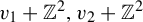
 $\mathcal R:{\mathcal {W}}\to (0,\infty )$
is given by
$\mathcal R:{\mathcal {W}}\to (0,\infty )$
is given by
 $$ \begin{align*}\mathcal R(\omega)=\min\{u>0: h_u (\omega)\in {\mathcal{W}}\}\end{align*} $$
and
 $T:{\mathcal {W}}\to {\mathcal {W}}$
is given by
$T:{\mathcal {W}}\to {\mathcal {W}}$
is given by
 $$ \begin{align*}\mathcal T(\omega) = h_{\mathcal R(\omega)}(\omega).\end{align*} $$
A simple, but key, observation is that the horocycle flow preserves slope differences of vectors
 $\vec {v}$
since
$\vec {v}$
since
 $$ \begin{align*}\text{slope}(h_u\vec{v})=\text{slope}(\vec{v})-u.\end{align*} $$
Consequently, this holds for holonomy vectors of saddle connections. This observation links slopes with
 ${\mathcal {W}}$
since if we apply horocycle flow to an element in
${\mathcal {W}}$
since if we apply horocycle flow to an element in
 ${\mathcal {W}}$
, we see that the next vector to become short is the vector with short horizontal component and smallest slope, and the return time to the Poincaré section is exactly its slope. Similarly, the second vector to become short will be the vector with short horizontal component and second smallest slope and the return time will be its slope minus the return time of the first, which is a slope difference. Continuing in this fashion, we see that the ith-return time is the difference of the
${\mathcal {W}}$
, we see that the next vector to become short is the vector with short horizontal component and smallest slope, and the return time to the Poincaré section is exactly its slope. Similarly, the second vector to become short will be the vector with short horizontal component and second smallest slope and the return time will be its slope minus the return time of the first, which is a slope difference. Continuing in this fashion, we see that the ith-return time is the difference of the
 $i{\textrm {th}}+1$
slope and the ith. This is formalized by
$i{\textrm {th}}+1$
slope and the ith. This is formalized by
 $$ \begin{align*}\mathcal R(\mathcal T^{{\kern2pt}i}(\omega)) = s_{i+1}-s_i.\end{align*} $$
Hence, we can relate our gap distribution to this induced dynamical system via
 $$ \begin{align} \frac{1}{N}|\mathcal G^N _V(\Lambda_\omega)\cap I|=\frac{1}{N}\sum_{i=0} ^{N-1}\chi_{\mathcal R^{-1}(I)}(\mathcal T^{{\kern2pt}i}(\Lambda_\omega)), \end{align} $$
where
 $\mathcal R^{-1}(I)$
is the set of slope differences in an interval I. Thus, the gap distribution reduces to understanding return times of
$\mathcal R^{-1}(I)$
is the set of slope differences in an interval I. Thus, the gap distribution reduces to understanding return times of
 ${\mathcal {W}}$
. The remainder of this paper will be concerned with computing the return times.
${\mathcal {W}}$
. The remainder of this paper will be concerned with computing the return times.
2.4 Moduli space
We introduce the moduli space of twice-marked tori and explain its connection to the space of doubled slit tori
 ${\mathcal {E}}$
.
${\mathcal {E}}$
.
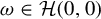
An example of a twice-marked torus. This is the standard torus of area 1 with marked points at the origin and at
 $(\tfrac {1}{2},{\pi }/{3})$
.
$(\tfrac {1}{2},{\pi }/{3})$
.
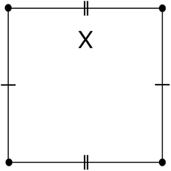
By a twice-marked torus, we simply mean a (unit area) torus with a preferred vertical direction and two marked points. We denote the set of all twice-marked tori by
 $\mathcal H{(0,0)}$
. Concretely, a twice-marked torus is given by the data of a torus
$\mathcal H{(0,0)}$
. Concretely, a twice-marked torus is given by the data of a torus
 ${\mathbb {C}}/g{\mathbb {Z}}^2$
, the flat metric
${\mathbb {C}}/g{\mathbb {Z}}^2$
, the flat metric
 $\,dz$
inherited from the complex plane, and two district marked points
$\,dz$
inherited from the complex plane, and two district marked points
 $v_1+{\mathbb {Z}}^2,v_2+{\mathbb {Z}}^2$
where
$v_1+{\mathbb {Z}}^2,v_2+{\mathbb {Z}}^2$
where
 $g\in {\textrm {SL}}_2({\mathbb {R}})$
. We will always assume that the first marked point is at the origin and denote the second marked point by v. Denote such an element by
$g\in {\textrm {SL}}_2({\mathbb {R}})$
. We will always assume that the first marked point is at the origin and denote the second marked point by v. Denote such an element by
 ${\mathbb {T}}^2 _{g,v}$
. To each
${\mathbb {T}}^2 _{g,v}$
. To each
 ${\mathbb {T}}^2_{g,v}$
, we can associate the affine lattice given by the orbit of v under the lattice
${\mathbb {T}}^2_{g,v}$
, we can associate the affine lattice given by the orbit of v under the lattice
 $g{\mathbb {Z}}^2$
,
$g{\mathbb {Z}}^2$
,
 $$ \begin{align*}g{\mathbb{Z}}^2 + v.\end{align*} $$
Denote the space of all affine lattices by
 $AX_2.$
Given an affine lattice
$AX_2.$
Given an affine lattice
 $g{\mathbb {Z}}^2+v$
and taking its quotient by
$g{\mathbb {Z}}^2+v$
and taking its quotient by
 $g{\mathbb {Z}}^2$
yields a twice-marked torus
$g{\mathbb {Z}}^2$
yields a twice-marked torus
 ${\mathbb {T}}^2 _{g,v}$
. It is easy to see that these operations are inverses and so there is a bijection between the space of twice-marked tori
${\mathbb {T}}^2 _{g,v}$
. It is easy to see that these operations are inverses and so there is a bijection between the space of twice-marked tori
 $\mathcal H(0,0)$
and the space of affine lattices
$\mathcal H(0,0)$
and the space of affine lattices
 $AX_2.$
Recall the affine action of
 ${\textrm {SL}}_2({\mathbb {R}})\ltimes {\mathbb {R}}^2$
on
${\textrm {SL}}_2({\mathbb {R}})\ltimes {\mathbb {R}}^2$
on
 ${\mathbb {R}}^2$
given by
${\mathbb {R}}^2$
given by
 $(h,w)\cdot v = hv + w$
. Thus, we can consider the natural action of
$(h,w)\cdot v = hv + w$
. Thus, we can consider the natural action of
 ${\textrm {SL}}_2({\mathbb {R}})\ltimes {\mathbb {R}}^2$
on
${\textrm {SL}}_2({\mathbb {R}})\ltimes {\mathbb {R}}^2$
on
 $AX_2$
defined by
$AX_2$
defined by
 $$ \begin{align*}(h,w)\cdot (g{\mathbb{Z}}^2 + v) = (hg){\mathbb{Z}}^2 + (h v + w).\end{align*} $$
Note that
 ${\textrm {SL}}_2({\mathbb {R}})\ltimes {\mathbb {R}}^2$
acts transitively on
${\textrm {SL}}_2({\mathbb {R}})\ltimes {\mathbb {R}}^2$
acts transitively on
 $AX_2$
and that the stabilizer of
$AX_2$
and that the stabilizer of
 ${\mathbb {Z}}^2$
is given by
${\mathbb {Z}}^2$
is given by
 ${\textrm {SL}}_2({\mathbb {Z}})\ltimes {\mathbb {Z}}^2$
. Thus, we may identify
${\textrm {SL}}_2({\mathbb {Z}})\ltimes {\mathbb {Z}}^2$
. Thus, we may identify
 $AX_2$
(and hence
$AX_2$
(and hence
 $\mathcal H(0,0)$
) as the homogenous space
$\mathcal H(0,0)$
) as the homogenous space
 $$ \begin{align*}\mathcal H(0,0)=AX_2={\textrm{SL}}_2({\mathbb{R}})\ltimes {\mathbb{R}}^2/ {\textrm{SL}}_2({\mathbb{Z}})\ltimes {\mathbb{Z}}^2.\end{align*} $$
We denote an element in any of the above spaces (and hence all) by
 $(g,v)$
and leave the coset implicitly defined. Denote by
$(g,v)$
and leave the coset implicitly defined. Denote by
 $X_2$
the space of lattices which we can identify with the homogeneous space
$X_2$
the space of lattices which we can identify with the homogeneous space
 $$ \begin{align*}X_2 = {\textrm{SL}}_2({\mathbb{R}})/{\textrm{SL}}_2({\mathbb{Z}}).\end{align*} $$
There is the projection map
 $\mathcal H(0,0)=AX_2\to X_2$
given by
$\mathcal H(0,0)=AX_2\to X_2$
given by
 $(g,v)\mapsto g$
. This will be a torus bundle since the fiber of a point
$(g,v)\mapsto g$
. This will be a torus bundle since the fiber of a point
 $g{\mathbb {Z}}^2$
in
$g{\mathbb {Z}}^2$
in
 $X_2$
is a vector
$X_2$
is a vector
 $ v$
that is only defined up to
$ v$
that is only defined up to
 $g{\mathbb {Z}}^2$
and hence we think of v as living in the torus
$g{\mathbb {Z}}^2$
and hence we think of v as living in the torus
 ${\mathbb {R}}^2/g{\mathbb {Z}}^2$
.
${\mathbb {R}}^2/g{\mathbb {Z}}^2$
.
Recall, that
 ${\mathcal {E}}$
is the family of translation surfaces obtained by gluing two identical tori along a slit. Every such surface projects to a twice-marked torus by restricting to one torus and forgetting the slit. By reversing this process, we can obtain a doubled slit torus from a twice-marked torus, although some care must be taken. Indeed, suppose we have an element in
${\mathcal {E}}$
is the family of translation surfaces obtained by gluing two identical tori along a slit. Every such surface projects to a twice-marked torus by restricting to one torus and forgetting the slit. By reversing this process, we can obtain a doubled slit torus from a twice-marked torus, although some care must be taken. Indeed, suppose we have an element in
 $\mathcal H(0,0)$
which depends on the data
$\mathcal H(0,0)$
which depends on the data
 $g\in {\textrm {SL}}_2({\mathbb {R}})$
and
$g\in {\textrm {SL}}_2({\mathbb {R}})$
and
 $v\in {\mathbb {C}}/g{\mathbb {Z}}^2$
. We can take two copies of it and then consider a slit between the marked points to construct an element
$v\in {\mathbb {C}}/g{\mathbb {Z}}^2$
. We can take two copies of it and then consider a slit between the marked points to construct an element
 $\omega = \omega _{(g,v)}$
in
$\omega = \omega _{(g,v)}$
in
 ${\mathcal {E}}.$
There are four oriented trajectories between the marked points that we can choose corresponding to the ‘corners’ of the fundamental domain of
${\mathcal {E}}.$
There are four oriented trajectories between the marked points that we can choose corresponding to the ‘corners’ of the fundamental domain of
 ${\mathbb {C}}/g{\mathbb {Z}}^2$
spanned by the columns of g. Hence, each pair
${\mathbb {C}}/g{\mathbb {Z}}^2$
spanned by the columns of g. Hence, each pair
 $(g,v)\in \mathcal H(0,0)$
gives rise to four elements in
$(g,v)\in \mathcal H(0,0)$
gives rise to four elements in
 ${\mathcal {E}}$
, which is to say there is a degree-four map
${\mathcal {E}}$
, which is to say there is a degree-four map
 $$ \begin{align*}\Pi:{\mathcal{E}}\to\mathcal H(0,0)\end{align*} $$
given by ‘forgetting the slit’. Any time
 $\Pi (\omega )=(g,v)$
, we use the notation
$\Pi (\omega )=(g,v)$
, we use the notation
 $\omega = \omega _{(g,v)}$
. Since the degree of
$\omega = \omega _{(g,v)}$
. Since the degree of
 $\Pi $
is four, then
$\Pi $
is four, then
 ${\mathcal {E}}$
can be identified as four copies of
${\mathcal {E}}$
can be identified as four copies of
 $\mathcal H(0,0)$
, one copy for each oriented trajectory between the marked points.
$\mathcal H(0,0)$
, one copy for each oriented trajectory between the marked points.
Ultimately, we are interested in saddle connections of elements in
 ${\mathcal {E}}$
and one way to find saddle connections of a doubled slit torus is to look for trajectories between marked points of the twice-marked torus. This explains our interest in
${\mathcal {E}}$
and one way to find saddle connections of a doubled slit torus is to look for trajectories between marked points of the twice-marked torus. This explains our interest in
 $\mathcal H (0,0)$
.
$\mathcal H (0,0)$
.
2.5 Gap distribution for twice-marked tori
We also consider the gap distribution of twice-marked tori
 $\mathcal H(0,0)$
. However, instead of considering all trajectories between marked points, we will only be interested in those between distinct marked points with a specific orientation. The reason for this is because these trajectories define an affine lattice.
$\mathcal H(0,0)$
. However, instead of considering all trajectories between marked points, we will only be interested in those between distinct marked points with a specific orientation. The reason for this is because these trajectories define an affine lattice.
Let
 $\Lambda _\omega ^{d,+}$
denote the holonomies of trajectories that start at the origin and end at the other marked point. Let
$\Lambda _\omega ^{d,+}$
denote the holonomies of trajectories that start at the origin and end at the other marked point. Let
 $\mathcal S_V (\Lambda _\omega ^{d,+}) $
denote the set of slopes of holonomy vectors in the vertical strip V. Then as before, we can order them
$\mathcal S_V (\Lambda _\omega ^{d,+}) $
denote the set of slopes of holonomy vectors in the vertical strip V. Then as before, we can order them
 $$ \begin{align*}\mathcal S_V (\Lambda_\omega ^{d,+}) = \{0=s_0<s_1<\cdots<s_N<\cdots\}.\end{align*} $$
Let
 $\mathcal S_V ^N$
denote the first N slopes. We can associate to these slopes the set of gaps
$\mathcal S_V ^N$
denote the first N slopes. We can associate to these slopes the set of gaps
 $$ \begin{align*}\mathcal G^N _V(\Lambda_\omega ^d) = \{s_i-s_{i-1}\mid i = 1,\ldots, N \} \end{align*} $$
and consider a gap distribution question for the slopes in the vertical strip V
 $$ \begin{align*}\lim_{N\to\infty}\frac{| \mathcal G^N _V(\Lambda_\omega ^{d,+}) \cap I|}{N} \end{align*} $$
for an interval
 $I.$
We prove the following.
$I.$
We prove the following.
Theorem 2.2. There is a limiting probability density function
 $ g : [0,\infty ) \to [0,\infty )$
, with
$ g : [0,\infty ) \to [0,\infty )$
, with
 $$ \begin{align*}\lim_{N\to\infty}\frac{| \mathcal G^N _V(\Lambda_\omega ^{d,+}) \cap I|}{N}=\int_I g(x)\,dx\end{align*} $$
for almost every twice-marked torus
 $\omega \in \mathcal H(0,0)$
with respect to an
$\omega \in \mathcal H(0,0)$
with respect to an
 ${\textrm {SL}}_2({\mathbb {R}})$
-invariant probability measure on
${\textrm {SL}}_2({\mathbb {R}})$
-invariant probability measure on
 ${\mathcal {H}}(0,0)$
that is in the same measure class as the Lebesgue measure.
${\mathcal {H}}(0,0)$
that is in the same measure class as the Lebesgue measure.
In fact, we prove that the slope gap distribution for twice-marked tori always exists, but is not always the same. This is done by proving a measure classification result for the transversal under the map induced by horocycle flow (see §4.1). The gap distribution density is the same for twice-marked tori that are in the support of the same measure.
Moreover, if
 $\omega \in \mathcal H(0,0)$
corresponds to
$\omega \in \mathcal H(0,0)$
corresponds to
 $(g,v)\in AX_2$
, then
$(g,v)\in AX_2$
, then
 $\Lambda _\omega ^{d,+}$
is the affine lattice
$\Lambda _\omega ^{d,+}$
is the affine lattice
 $g{\mathbb {Z}}^2+v$
. See §3.2.1 for a detailed discussion on this. Hence, the above theorem can be interpreted as a theorem about gaps of slopes of an affine lattice. The distribution of gaps of angles of affine lattices was studied in [Reference Marklof and Strömbergsson17]. They show that the gap distribution agrees with the distribution of gaps of the sequence
$g{\mathbb {Z}}^2+v$
. See §3.2.1 for a detailed discussion on this. Hence, the above theorem can be interpreted as a theorem about gaps of slopes of an affine lattice. The distribution of gaps of angles of affine lattices was studied in [Reference Marklof and Strömbergsson17]. They show that the gap distribution agrees with the distribution of gaps of the sequence
 $(\sqrt {n})_{n\in {\mathbb {N}}}$
on the unit circle found by Elkies and McMullen [Reference Elkies and McMullen10].
$(\sqrt {n})_{n\in {\mathbb {N}}}$
on the unit circle found by Elkies and McMullen [Reference Elkies and McMullen10].
A consequence of Theorem 2.2 is that the gap distribution of affine lattices has a quadratic tail and hence is not exotic (Theorem 4.4(1)). As with the gap distribution of doubled slit tori, we prove much finer results, but we wait until §4 Theorem 4.4 before more precisely stating them. Our proof technique is the same as for doubled slit tori, namely, we translate the gap distribution question to one of return times to a transversal on the moduli space of twice-marked tori
 $\mathcal H(0,0).$
The explicit computation of these return times addresses a question from [Reference Athreya2, §6.2].
$\mathcal H(0,0).$
The explicit computation of these return times addresses a question from [Reference Athreya2, §6.2].
The transversal we consider is given by the set of twice-marked tori that have a horizontal saddle connection that starts at the origin and ends at the other marked point with a length less than or equal to 1. Denote this set by
 $\Omega $
. Thus,
$\Omega $
. Thus,
 $$ \begin{align*}\Omega =\{\omega\in \mathcal H(0,0): \Lambda_\omega ^{d,+}\cap (0,1]\ne \emptyset \}.\end{align*} $$
Under the identification of
 $\mathcal H(0,0)$
and
$\mathcal H(0,0)$
and
 $AX_2$
,
$AX_2$
,
 $\Omega $
is the same as the set of affine lattices that contain a non-zero horizontal vector with horizontal component less than or equal to 1. That is,
$\Omega $
is the same as the set of affine lattices that contain a non-zero horizontal vector with horizontal component less than or equal to 1. That is,
 $\Omega $
can be identified with
$\Omega $
can be identified with
 $$ \begin{align*}\{\Lambda \in AX_2: \Lambda\cap (0,1]\ne \emptyset\}.\end{align*} $$
We will abuse notation and refer to the above set as
 $\Omega $
. The set
$\Omega $
. The set
 $\Omega \subset \mathcal H(0,0)$
is a transversal for horocycle flow. We postpone proof of these statements until §3. We will call a horizontal vector with a horizontal component less than or equal to one a short vector and an element in
$\Omega \subset \mathcal H(0,0)$
is a transversal for horocycle flow. We postpone proof of these statements until §3. We will call a horizontal vector with a horizontal component less than or equal to one a short vector and an element in
 $\Omega $
a short affine lattice.
$\Omega $
a short affine lattice.
Henceforth, we will only think about elements
 $(g,v)$
as affine lattices. Furthermore, unless explicitly stated, we will assume that for an element
$(g,v)$
as affine lattices. Furthermore, unless explicitly stated, we will assume that for an element
 $(g,v)\in \mathcal H(0,0)$
or
$(g,v)\in \mathcal H(0,0)$
or
 $\omega _{(g,v)}\in \mathcal E$
, we have
$\omega _{(g,v)}\in \mathcal E$
, we have
 $v\notin g{\mathbb {Q}}^2$
. This assumption only removes a set of measure zero elements from our spaces and, since we are concerned only with almost everywhere results, is a mild one.
$v\notin g{\mathbb {Q}}^2$
. This assumption only removes a set of measure zero elements from our spaces and, since we are concerned only with almost everywhere results, is a mild one.
3 Parameterization of the transversal and return times
We give coordinates to the transversals from the last section and compute the first return time under these coordinates.
3.1 On twice-marked tori
 $\mathcal H(0,0)$

Here, we parameterize our Poincaré section
 $\Omega $
and compute the first return time to
$\Omega $
and compute the first return time to
 $\Omega $
. We also recall some results from [Reference Athreya and Cheung5] that will aid us.
$\Omega $
. We also recall some results from [Reference Athreya and Cheung5] that will aid us.
3.1.1 A Poincaré section for
$X_2$

Before parameterizing our section, we recall some results from [Reference Athreya and Cheung5] where they considered a Poincaré section for
 $X_2$
, which they used to obtain statistical properties of Farey fractions. We fix the notation
$X_2$
, which they used to obtain statistical properties of Farey fractions. We fix the notation
 $$ \begin{align*}p_{a,b} := \left( \begin{array}{ c c } a & b \\ 0 & a^{-1} \end{array} \right)\end{align*} $$
and
 $$ \begin{align*}g_{t} := \left( \begin{array}{ c c } e^{t} & 0 \\ 0 & e^{-t} \end{array} \right).\end{align*} $$
Let
 $\Delta $
denote the set of lattices that contains a short vector (recall that short for us means length less than or equal to
$\Delta $
denote the set of lattices that contains a short vector (recall that short for us means length less than or equal to
 $1$
). It is shown in [Reference Athreya and Cheung5] that this set is
$1$
). It is shown in [Reference Athreya and Cheung5] that this set is
 $$ \begin{align*}\Delta = \left\{\Lambda_{a,b} := p_{a,b}{\mathbb{Z}}^2 = \left( \begin{array}{ c c } a & b \\ 0 & a^{-1} \end{array} \right) {\mathbb{Z}}^2 : 0<a\le1, 1-a<b\le1\right\}.\end{align*} $$
There is a bijection between
 $\Delta $
with the actual triangle
$\Delta $
with the actual triangle
 $$ \begin{align*}\{(a,b):0<a\le1, 1-a<b\le1\}\subset {\mathbb{R}}^2\end{align*} $$
via
 $(a,b)\mapsto \Lambda _{a,b}$
and thus we give an element in
$(a,b)\mapsto \Lambda _{a,b}$
and thus we give an element in
 $\Lambda _{a,b}\in \Delta $
the coordinates
$\Lambda _{a,b}\in \Delta $
the coordinates
 $(a,b)$
. Because of the bijection, we abuse notation and use
$(a,b)$
. Because of the bijection, we abuse notation and use
 $\Delta $
for the subset of
$\Delta $
for the subset of
 $X_2$
and the actual triangle.
$X_2$
and the actual triangle.
We now restate the main theorem [Reference Athreya and Cheung5, Theorem 1.1] with slightly different notation.
Theorem 3.1. The subset
 $\Delta \subset X_2$
is a Poincaré section for the horocycle action on
$\Delta \subset X_2$
is a Poincaré section for the horocycle action on
 $X_2$
. More precisely, every horocycle orbit
$X_2$
. More precisely, every horocycle orbit
 $\{h_s \Lambda \}_{s\in {\mathbb {R}}}$
(outside a codimension
$\{h_s \Lambda \}_{s\in {\mathbb {R}}}$
(outside a codimension
 $1$
set of lattices) intersects
$1$
set of lattices) intersects
 $\Delta $
in a non-empty, countable, discrete set of times.
$\Delta $
in a non-empty, countable, discrete set of times.
Moreover, the first return time map
 $r:\Delta \to [0,\infty )$
is given by
$r:\Delta \to [0,\infty )$
is given by
 $$ \begin{align*}r(\Lambda_{a,b})=r(a,b)=\min\{s>0: h_s\Lambda_{a,b}\in \Delta\}=(ab)^{-1}\end{align*} $$
and the return map
 $S:\Delta \to \Delta $
is
$S:\Delta \to \Delta $
is
 $$ \begin{align*}S(\Lambda_{a,b}):=h_{r(a,b)}\Lambda_{a,b}:=\Lambda_{S(a,b)}\end{align*} $$
where
 $S(a,b)=(b,-a+\lfloor ({1+a})/{b}\rfloor b)$
.
$S(a,b)=(b,-a+\lfloor ({1+a})/{b}\rfloor b)$
.
They also identify the codimension
 $1$
set as those lattices that contain a short vertical vector, which geometrically correspond to embedded closed horocycles that foliate the cusp. Dynamically, for any
$1$
set as those lattices that contain a short vertical vector, which geometrically correspond to embedded closed horocycles that foliate the cusp. Dynamically, for any
 $0<a\le 1$
, each horocycle is a periodic orbit under horocycle flow
$0<a\le 1$
, each horocycle is a periodic orbit under horocycle flow
 $h_s$
with period
$h_s$
with period
 $a^{2}$
and orbit
$a^{2}$
and orbit
 $$ \begin{align*}\text{Per}(a):=\left\{ h_sg_{\log(a)} {\mathbb{Z}}^2= \left( \begin{array}{ c c } 0 & -a^{-1} \\ a & sa^{-1} \end{array} \right){\mathbb{Z}}^2:s\in[0,a^2)\right\}.\end{align*} $$
Notice above, we implicitly used that
 $$ \begin{align*}h_sg_{\log(a)} {\mathbb{Z}}^2=h_sg_{\log(a)} \left( \begin{array}{ c c } 0 & -1 \\ 1 & 0 \end{array} \right) {\mathbb{Z}}^2 = \left( \begin{array}{ c c } 0 & -a^{-1} \\ a & sa^{-1} \end{array} \right){\mathbb{Z}}^2\end{align*} $$
so as to further drive the point that such elements are outside of the generic set of lattices. Of course, any
 $a>0$
gives rise to a periodic orbit
$a>0$
gives rise to a periodic orbit
 $\text {Per}(a)$
, but only the
$\text {Per}(a)$
, but only the
 $0<a\le 1$
give rise to points that never enter the transversal
$0<a\le 1$
give rise to points that never enter the transversal
 $\Delta .$
As a consequence of their theorem, we have that every
 $g\in X_2$
is one of the two forms.
$g\in X_2$
is one of the two forms.
-
(1)
$g=h_sp_{a,b}$
, where
$0<a\le 1$
,
$1-a<b\le 1$
, and
$0\le s<(ab)^{-1}$
. These are the generic elements in
$X_2$
. -
(2)
$g = h_sg_{\log (a)}$
, where
$0\le a<1$
and
$0\le s<a^2$
. These are the elements in the codimension
$1$
set of lattices with a short vertical vector.


3.1.2 A Poincaré section for
$AX_2$

In this section, we show
 $\Omega $
is indeed a transversal and give coordinates to
$\Omega $
is indeed a transversal and give coordinates to
 $\Omega .$
Observe that since the dimension of the space of affine lattices
$\Omega .$
Observe that since the dimension of the space of affine lattices
 $AX_2$
is five, the cross-section by horocycle flow will have dimension equal to four. Thus, we aim to find a four-dimensional parameterization.
$AX_2$
is five, the cross-section by horocycle flow will have dimension equal to four. Thus, we aim to find a four-dimensional parameterization.
We prove a lemma that says that any affine lattice
 $(g,v)\in \Omega $
can be expressed as an affine lattice where the affine piece is horizontal.
$(g,v)\in \Omega $
can be expressed as an affine lattice where the affine piece is horizontal.
Lemma 3.2. The set of short affine lattices is given by
 $$ \begin{align*}\Omega=\left\{(g,v)\in AX_2: v= \left( \begin{array}{ c c } {\alpha} \\ 0 \end{array} \right) \text{ and }{\alpha}\in(0,1]\right\}.\end{align*} $$
Proof Suppose that
 $(g,v)\in \Omega $
, that is that the affine lattice
$(g,v)\in \Omega $
, that is that the affine lattice
 $(g,v)$
contains a short horizontal vector. Recall that v is only defined up to elements in
$(g,v)$
contains a short horizontal vector. Recall that v is only defined up to elements in
 $g{\mathbb {Z}}^2$
. Hence, if
$g{\mathbb {Z}}^2$
. Hence, if
 $ w\in g{\mathbb {Z}}^2$
, then as an affine lattice, we have
$ w\in g{\mathbb {Z}}^2$
, then as an affine lattice, we have
 $$ \begin{align*}g{\mathbb{Z}}^2 + v =g{\mathbb{Z}}^2 + ( v +w) .\end{align*} $$
In particular, if we assume our affine lattice is short, then there is some
 $ w\in g{\mathbb {Z}}^2$
so that
$ w\in g{\mathbb {Z}}^2$
so that
 $w+ v$
is a short horizontal vector. In particular, it is of the form
$w+ v$
is a short horizontal vector. In particular, it is of the form
 $$ \begin{align*}w+v = \left( \begin{array}{ c c } {\alpha} \\ 0 \end{array} \right)\end{align*} $$
for some
 ${\alpha }\in (0,1]$
. Thus,
${\alpha }\in (0,1]$
. Thus,
 $$ \begin{align*}g{\mathbb{Z}}^2 + v =g{\mathbb{Z}}^2 + v +w = g{\mathbb{Z}}^2 +\left( \begin{array}{ c c } {\alpha} \\ 0 \end{array} \right).\\[-40pt]\end{align*} $$
Armed with the above lemma, we also provide proof of our claims from the previous section.
Lemma 3.3. Under the identification of
 $\mathcal H(0,0)$
and
$\mathcal H(0,0)$
and
 $AX_2$
, we have that
$AX_2$
, we have that
 $$ \begin{align*}\{\omega\in \mathcal H(0,0): \Lambda_\omega ^{d,+}\cap (0,1]\ne \emptyset \}\end{align*} $$
is the same as the set of affine lattices that contain a non-zero horizontal vector with horizontal component less than or equal to
 $1$
,
$1$
,
 $$ \begin{align*}\{\Lambda \in AX_2: \Lambda\cap (0,1]\ne \emptyset\}.\end{align*} $$
Proof This follows from the identification of
 $\mathcal H(0,0)$
and
$\mathcal H(0,0)$
and
 $AX_2$
and use of Proposition 3.9 that yields if
$AX_2$
and use of Proposition 3.9 that yields if
 $\omega \in \mathcal H(0,0)$
is the twice-marked torus formed by
$\omega \in \mathcal H(0,0)$
is the twice-marked torus formed by
 $(g,v)$
, then
$(g,v)$
, then
 $\Lambda _\omega ^{d,+}=g{\mathbb {Z}}^2+v$
.
$\Lambda _\omega ^{d,+}=g{\mathbb {Z}}^2+v$
.
If
 $\omega \in \Omega $
with short horizontal saddle connection
$\omega \in \Omega $
with short horizontal saddle connection
 $\gamma $
with holonomy in
$\gamma $
with holonomy in
 $\Lambda _\omega ^{d,+}$
, then tiling
$\Lambda _\omega ^{d,+}$
, then tiling
 ${\mathbb {C}}$
by a fundamental domain of
${\mathbb {C}}$
by a fundamental domain of
 $\omega $
produces an affine lattice with a short horizontal vector given by the holonomy of
$\omega $
produces an affine lattice with a short horizontal vector given by the holonomy of
 $\gamma .$
Conversely, if we are given an affine lattice
$\gamma .$
Conversely, if we are given an affine lattice
 $\Lambda $
with
$\Lambda $
with
 $\Lambda \cap (0,1]\ne \emptyset $
, then we can assume the affine part is producing the vector in
$\Lambda \cap (0,1]\ne \emptyset $
, then we can assume the affine part is producing the vector in
 $(0,1]$
by the previous lemma. That is, we can assume
$(0,1]$
by the previous lemma. That is, we can assume
 $$ \begin{align*}\Lambda = g{\mathbb{Z}}^2 + \left(\begin{array}{ c c } {\alpha} \\ 0 \end{array}\right)\end{align*} $$
for
 $\alpha \in (0,1]$
. Taking the quotient by
$\alpha \in (0,1]$
. Taking the quotient by
 $g{\mathbb {Z}}^2$
produces a twice-marked torus along with a saddle connection
$g{\mathbb {Z}}^2$
produces a twice-marked torus along with a saddle connection
 $\gamma $
that has holonomy
$\gamma $
that has holonomy
 $(\begin {smallmatrix} {\alpha } \\ 0 \end {smallmatrix})$
.
$(\begin {smallmatrix} {\alpha } \\ 0 \end {smallmatrix})$
.
Lemma 3.4. The set
 $\Omega $
is a transversal for horocycle flow. That is, almost every orbit under horocycle flow intersects
$\Omega $
is a transversal for horocycle flow. That is, almost every orbit under horocycle flow intersects
 $\Omega $
in a non-empty, countable, discrete set of times.
$\Omega $
in a non-empty, countable, discrete set of times.
Proof This follows along the same lines of justification as Lemma 2.1 of Athreya [Reference Athreya2] and the discussion in §2.3. Notice that generically an affine lattice
 $\Lambda \in AX_2$
has infinitely many vectors contained in the vertical strip
$\Lambda \in AX_2$
has infinitely many vectors contained in the vertical strip
 $V = \{(x,y)\in {\mathbb {R}}^2:0< x\le 1, y>0\}$
. Then,
$V = \{(x,y)\in {\mathbb {R}}^2:0< x\le 1, y>0\}$
. Then,
 $h_u\Lambda \in \Omega $
exactly when u is the slope of the smallest vector contained
$h_u\Lambda \in \Omega $
exactly when u is the slope of the smallest vector contained
 $\Lambda \cap V$
. Similarly,
$\Lambda \cap V$
. Similarly,
 $h_{u'}h_{u}\Lambda \in \Omega $
when
$h_{u'}h_{u}\Lambda \in \Omega $
when
 $u'$
is the slope of the smallest vector contained
$u'$
is the slope of the smallest vector contained
 $h_{u}(\Lambda )\cap V$
. This shows almost every orbit under horocycle flow intersects
$h_{u}(\Lambda )\cap V$
. This shows almost every orbit under horocycle flow intersects
 $\Omega $
in a non-empty, countable set of times. These intersections have to happen at discrete times since
$\Omega $
in a non-empty, countable set of times. These intersections have to happen at discrete times since
 $\Lambda $
itself is discrete.
$\Lambda $
itself is discrete.
We use this lemma along with the coordinates on the space of lattices developed in [Reference Athreya and Cheung5] to parameterize
 $\Omega $
.
$\Omega $
.
Proposition 3.5. The set of of short affine lattices is given by the union of
 $$ \begin{align*}\left\{\left(h_sp_{a,b}, \left( \begin{array}{ c c } {\alpha} \\ 0 \end{array} \right)\right) :a\in(0,1], b\in(1-a,1], s\in\left[0,(ab)^{-1}\right),\alpha\in(0,1])\right\}\end{align*} $$
and
 $$ \begin{align*}\left\{\left(h_sg_{\log(a)}, \left( \begin{array}{ c c } {\alpha} \\ 0 \end{array} \right)\right) :a\in(0,1],s\in(0,a^2],\alpha\in(0,1])\right\}.\end{align*} $$
Proof First notice that any affine lattice from the union is a short affine lattice.
Now suppose
 $(g,v)\in \Omega $
. By the last lemma, we can assume v is a short vector. Combining this with the coordinates developed in [Reference Athreya and Cheung5], which we recalled in the last section, we can finish the proof of our parameterization. By the results of [Reference Athreya and Cheung5], a generic lattice
$(g,v)\in \Omega $
. By the last lemma, we can assume v is a short vector. Combining this with the coordinates developed in [Reference Athreya and Cheung5], which we recalled in the last section, we can finish the proof of our parameterization. By the results of [Reference Athreya and Cheung5], a generic lattice
 $g{\mathbb {Z}}^2\in X_2$
(of a codimension
$g{\mathbb {Z}}^2\in X_2$
(of a codimension
 $1$
set) has the form
$1$
set) has the form
 $$ \begin{align*}g{\mathbb{Z}}^2=h_s p_{a,b}{\mathbb{Z}}^2=\left( \begin{array}{ c c } a & b \\ -sa & a^{-1}-sb \end{array} \right){\mathbb{Z}}^2\end{align*} $$
with
 $0<a\le 1$
,
$0<a\le 1$
,
 $1-a<b\le 1$
, and
$1-a<b\le 1$
, and
 $0<s<(ab)^{-1}$
.
$0<s<(ab)^{-1}$
.
Thus, we can give such an element in
 $(g,v)\in \Omega $
the coordinates
$(g,v)\in \Omega $
the coordinates
 $(a,b,s,\alpha )$
, where
$(a,b,s,\alpha )$
, where
 $$ \begin{align*}g{\mathbb{Z}}^2=h_s p_{a,b}{\mathbb{Z}}^2 \text{ and }v=\left( \begin{array}{ c c } {\alpha} \\ 0 \end{array} \right).\end{align*} $$
If g is in the codimension
 $1$
set, then it is of the form
$1$
set, then it is of the form
 $$ \begin{align*}g{\mathbb{Z}}^2=h_sg_{\log(a)}{\mathbb{Z}}^2=\left( \begin{array}{ c c } 0 & -a^{-1} \\ a & sa^{-1} \end{array} \right){\mathbb{Z}}^2\end{align*} $$
with
 $0<a\le 1$
, and
$0<a\le 1$
, and
 $0<s<a^2$
, and we give it the coordinates
$0<s<a^2$
, and we give it the coordinates
 $(a,s,{\alpha }).$
We note that the affine lattice
 $(a,0,s,{\alpha })$
is not the same as the affine lattice
$(a,0,s,{\alpha })$
is not the same as the affine lattice
 $(a,s,{\alpha })$
.
$(a,s,{\alpha })$
.
3.1.3 First return time to
$\Omega $

As mentioned above, our goal is to find the return map to our transversal, which will calculate the gap distribution for slopes in the vertical strip V. We outline the strategy of how to do this: If we had the point
 $(g,v)\in \Omega $
that is an affine lattice with a short horizontal vector, then we have
$(g,v)\in \Omega $
that is an affine lattice with a short horizontal vector, then we have
 $v=(\begin {smallmatrix} {\alpha } \\ 0 \end {smallmatrix})$
for some
$v=(\begin {smallmatrix} {\alpha } \\ 0 \end {smallmatrix})$
for some
 $0<\alpha \le 1$
. Choose any vector
$0<\alpha \le 1$
. Choose any vector
 $(\begin {smallmatrix} x \\ y \end {smallmatrix})\in g{\mathbb {Z}}^2$
. Then the horocycle flow action on the vectors of the affine lattice
$(\begin {smallmatrix} x \\ y \end {smallmatrix})\in g{\mathbb {Z}}^2$
. Then the horocycle flow action on the vectors of the affine lattice
 $(g,v)$
is given by
$(g,v)$
is given by
 $$ \begin{align*}h_u\left( \begin{array}{ c c } x \\ y \end{array} \right) + h_u\left( \begin{array}{ c c } {\alpha} \\ 0 \end{array} \right)=\left( \begin{array}{ c c } x+\alpha \\ y-u(x+\alpha) \end{array} \right).\end{align*} $$
Thus, if we want a short vector, then we need the horizontal
 $x+{\alpha }$
between 0 and 1,
$x+{\alpha }$
between 0 and 1,
 $y>0$
(so that
$y>0$
(so that
 $(x+{\alpha },y)$
is in the vertical strip), and
$(x+{\alpha },y)$
is in the vertical strip), and
 $$ \begin{align*}u=\frac{y}{x+\alpha}\end{align*} $$
so that the vertical is zero. As there are several lattice points that will meet this criteria and since we are seeking the first return time, we will minimize
 $u>0$
over all lattice points in
$u>0$
over all lattice points in
 $g{\mathbb {Z}}^2$
and the vertical strip V. Which is to say, we want to compute
$g{\mathbb {Z}}^2$
and the vertical strip V. Which is to say, we want to compute
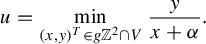 $$ \begin{align*}u=\min_{(x,y)^T\in g{\mathbb{Z}}^2\cap V}\frac{y}{x+\alpha}.\end{align*} $$
We can unpack a little more by observing that an element in a generic lattice has the form
 $g=h_sp_{a,b}$
, where
$g=h_sp_{a,b}$
, where
 $0<a\le 1$
,
$0<a\le 1$
,
 $1-a<b\le 1$
,
$1-a<b\le 1$
,
 $0\le s<{(ab)}^{-1},$
and
$0\le s<{(ab)}^{-1},$
and
 $0<\alpha \le 1$
.
$0<\alpha \le 1$
.
Thus, we are trying to find the minimum of the slopes of these vectors
 $$ \begin{align*}R(a,b,s,{\alpha}):= \min_{m,n\in {\mathbb{Z}}}\frac{(a^{-1}-sb)n - sam}{ma+nb + \alpha}\end{align*} $$
subject to the constraints:
-
(1)
$0<ma+nb + \alpha \le 1$
so that the horizontal is short; -
(2)
$ (a^{-1}-sb)n - sam$
is positive so that we are sampling points in the vertical strip V,

because this minimum is the return time. Our main result in this part is an explicit return time computation for generic affine lattices.
Theorem 3.6. Let
 $j=\lfloor ({1+a-\alpha })/{b}\rfloor $
. If
$j=\lfloor ({1+a-\alpha })/{b}\rfloor $
. If
 ${\alpha }>a$
, then
${\alpha }>a$
, then
 $$ \begin{align*}R(a,b,s,{\alpha}) = \begin{cases} \dfrac{sa}{{\alpha}-a} &\text{ if } s<\dfrac{{\alpha}-a}{ab{\alpha}},\\[5pt] \dfrac{j(a^{-1}-sb)+sa}{{\alpha}-a+jb} &\text{ if } s>\dfrac{{\alpha}-a}{ab{\alpha}}. \end{cases}\end{align*} $$
If
 ${\alpha }\le a$
, then
${\alpha }\le a$
, then
 $$ \begin{align*}R(a,b,s,{\alpha}) = \begin{cases} \dfrac{a^{-1}-sb}{b+{\alpha}} &\text{ if } b+{\alpha}\le1,\\[5pt] \dfrac{j(a^{-1}-sb)+sa}{{\alpha}-a+jb} &\text{ if } b+{\alpha}>1. \end{cases}\end{align*} $$
Proof The main idea is to notice that for any fixed n, there is a unique
 $m=m_n$
for which the affine lattice point
$m=m_n$
for which the affine lattice point
 $$ \begin{align*}\left( \begin{array}{ c c } ma+nb + \alpha \\ (a^{-1}-sb)n - sam \end{array} \right)\end{align*} $$
may be a candidate to minimize slope. From there, we can single out a candidate vector that provides an upper bound to the minimum slope and then use that candidate along with the structure of the affine lattice to find the actual minimum.
Fix
 $n\in {\mathbb {Z}}$
, if we have a candidate affine lattice point, then the horizontal must satisfy
$n\in {\mathbb {Z}}$
, if we have a candidate affine lattice point, then the horizontal must satisfy
 $$ \begin{align*}0<ma+nb + \alpha\le 1\iff \frac{-(nb+{\alpha})}{a}<m \le \frac{1-(nb+{\alpha})}{a}.\end{align*} $$
Since we require
 $m\in {\mathbb {Z}}$
, we have that m must be one of the following:
$m\in {\mathbb {Z}}$
, we have that m must be one of the following:
 $$ \begin{align*}\bigg\lceil \frac{-(nb+{\alpha})}{a}\bigg\rceil, \bigg\lceil \frac{-(nb+{\alpha})}{a}\bigg\rceil +1, \bigg\lceil \frac{-(nb+{\alpha})}{a}\bigg\rceil +2, \ldots, \bigg\lfloor \frac{1-(nb+{\alpha})}{a} \bigg\rfloor.\end{align*} $$
Now notice that to minimize the slope
 $$ \begin{align*}\frac{(a^{-1}-sb)n - sam}{ma+nb + \alpha},\end{align*} $$
we should maximize m. Hence, we choose
 $m_n = \lfloor ({1-(nb+{\alpha })})/{a} \rfloor $
. In particular, for every
$m_n = \lfloor ({1-(nb+{\alpha })})/{a} \rfloor $
. In particular, for every
 $n\in {\mathbb {Z}}$
, there is a single
$n\in {\mathbb {Z}}$
, there is a single
 $m=m_n$
for which the associated affine lattice point may be a minimizer.
$m=m_n$
for which the associated affine lattice point may be a minimizer.
Using this fact, we will single out a candidate and use the structure of the lattice to find the true minimum.
We proceed by cases.
Case 1:
 ${\alpha }<a$
. Consider the candidate minimizers when
${\alpha }<a$
. Consider the candidate minimizers when
 $n=1$
. Since their horizontal must be short, we deduce that
$n=1$
. Since their horizontal must be short, we deduce that
 $$ \begin{align*}0<ma + b + {\alpha} \le 1 \iff \frac{-(b+{\alpha})}{a}<m\le \frac{1-(b+{\alpha})}{a}.\end{align*} $$
Since we are trying to minimize the slope
 $({a^{-1}-sb - sam})/({ma+b+{\alpha }})$
, then we want to maximize m and so
$({a^{-1}-sb - sam})/({ma+b+{\alpha }})$
, then we want to maximize m and so
 $$ \begin{align*}m=\bigg\lfloor \frac{1-(b+{\alpha})}{a}\bigg\rfloor.\end{align*} $$
We claim that the only possible values for this floor are 0 and 1. Indeed, notice by our choice of coordinates we have
 $$ \begin{align*}1-a<b\le1 \iff{-\alpha} \le 1-(b+{\alpha})<a-{\alpha}.\end{align*} $$
An obvious upper bound is a and due to our assumption that
 ${\alpha }<a$
, we have that a lower bound is
${\alpha }<a$
, we have that a lower bound is
 $-a$
. Hence,
$-a$
. Hence,
 $$ \begin{align*}-a \le 1-(b+{\alpha})<a\iff {-1} \le \frac{1-(b+{\alpha})}{a}<1.\end{align*} $$
This proves the claim that
 $m\in \{0,1\}$
. Moreover, we see that
$m\in \{0,1\}$
. Moreover, we see that
 $$ \begin{align*}m=\bigg\lfloor \frac{1-(b+{\alpha})}{a}\bigg\rfloor = \begin{cases} 0 &\text{ if } b+{\alpha}\le 1,\\ -1 &\text{ if } b+{\alpha}>1.\\ \end{cases}\end{align*} $$
Hence, in the case that
 ${\alpha }<a$
, the candidate when
${\alpha }<a$
, the candidate when
 $n=1$
is
$n=1$
is
 $$ \begin{align*}\gamma_1:= \begin{cases} \left( \begin{array}{ c c } b+{\alpha} \\ a^{-1}-sb \end{array} \right) &\text{ if } b+{\alpha}\le1,\\ \left( \begin{array}{ c c } b + {\alpha} -a \\ a^{-1} -sb+sa \end{array} \right) &\text{ if } b+{\alpha}>1.\\ \end{cases}\end{align*} $$
Now, the minimum slope is bounded above by slope
 $(\gamma _1)$
and that to get any other candidate vector, we must add/subtract multiples of the basis vectors of
$(\gamma _1)$
and that to get any other candidate vector, we must add/subtract multiples of the basis vectors of
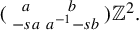 $(\begin {smallmatrix} a &b \\ -sa & a^{-1}-sb \end {smallmatrix}){\mathbb {Z}}^2.$
Recall we found
$(\begin {smallmatrix} a &b \\ -sa & a^{-1}-sb \end {smallmatrix}){\mathbb {Z}}^2.$
Recall we found
 $\gamma _1$
by fixing
$\gamma _1$
by fixing
 $n=1$
, this means that we cannot obtain any other candidates by adding/ subtracting the first basis vector. First notice that
$n=1$
, this means that we cannot obtain any other candidates by adding/ subtracting the first basis vector. First notice that
 $$ \begin{align*}\gamma_1 -\left( \begin{array}{ c c } b \\ a^{-1} -sb \end{array} \right)\end{align*} $$
has vertical zero so that it is not a candidate to minimize slope. Hence, to find other candidates to minimize slope, our only option to is to add the second basis vector
 $(\begin {smallmatrix} b \\ a^{-1} -sb \end {smallmatrix})$
to
$(\begin {smallmatrix} b \\ a^{-1} -sb \end {smallmatrix})$
to
 $\gamma _1$
to get the other candidates at different levels (as long as the horizontal is less than 1). For example, the level 2 candidate
$\gamma _1$
to get the other candidates at different levels (as long as the horizontal is less than 1). For example, the level 2 candidate
 $$ \begin{align*}\gamma_2=\gamma_1 + \left( \begin{array}{ c c } b \\ a^{-1} -sb \end{array} \right).\end{align*} $$
More generally, all of our candidates are
 $$ \begin{align*}\gamma_n=\gamma_1 + (n-1)\left( \begin{array}{ c c } b \\ a^{-1} -sb \end{array} \right),\end{align*} $$
where
 $n\ge 1$
and so long as the horizontal is less than 1. Of course, once the horizontal becomes bigger than 1, we subtract the other basis vector, but since we are decreasing the horizontal, we are increasing the slope so that we do not need to look at these candidates.
$n\ge 1$
and so long as the horizontal is less than 1. Of course, once the horizontal becomes bigger than 1, we subtract the other basis vector, but since we are decreasing the horizontal, we are increasing the slope so that we do not need to look at these candidates.
Now notice that
 $$ \begin{align*}\begin{cases} \text{ if } b+{\alpha}\le1, \text{ adding } \left( \begin{array}{ c c } b \\ a^{-1} -sb \end{array} \right) \text{ to}\ \gamma_1\ \text{increases slope}, \\ \text{ if } b+{\alpha}>1,\text{ adding } \left( \begin{array}{ c c } b \\ a^{-1} -sb \end{array} \right) \text{ to}\ \gamma_1\ \text{decreases slope}.\\ \end{cases}\end{align*} $$
We conclude that the return time is
 $$ \begin{align*}\begin{cases} \text{ slope }(\gamma_1) \text{ if } b+{\alpha}\le1,\\ \text{ slope }(\gamma_j) \text{ if } b+{\alpha}>1, \\ \end{cases}\end{align*} $$
where j is the maximum number of times we can add
 $(\begin {smallmatrix} b \\ a^{-1} -sb \end {smallmatrix})$
to
$(\begin {smallmatrix} b \\ a^{-1} -sb \end {smallmatrix})$
to
 $\gamma _1$
so that the horizontal of
$\gamma _1$
so that the horizontal of
 $\gamma _j$
is smaller than 1. We compute this value of j: This is the largest number so that
$\gamma _j$
is smaller than 1. We compute this value of j: This is the largest number so that
 $$ \begin{align*}\text{ horizontal }(\gamma_j) = jb+\alpha -a \le 1<(j+1)b+\alpha -a \iff j=\bigg \lfloor \frac{a+1-\alpha}{b}\bigg\rfloor.\end{align*} $$
Case 2:
 $a<{\alpha }$
. This case is slightly easier since we have a candidate at
$a<{\alpha }$
. This case is slightly easier since we have a candidate at
 $n=0$
given by
$n=0$
given by
 $$ \begin{align*}\gamma_0 = \left( \begin{array}{ c c } {\alpha} \\ 0 \end{array} \right) - \left( \begin{array}{ c c } a \\ -sa \end{array} \right) = \left( \begin{array}{ c c } {\alpha} - a \\ sa \end{array} \right).\end{align*} $$
This candidate is in the vertical strip V by our assumption
 $a< {\alpha }$
and does not exist in Case 1. Notice that subtracting the second basis vector will yield a negative horizontal.
$a< {\alpha }$
and does not exist in Case 1. Notice that subtracting the second basis vector will yield a negative horizontal.
Now, as before, to obtain any other candidate, all we can do is add the second basis vector yielding the candidates
 $$ \begin{align*}\gamma_n = \gamma_0 + n\left( \begin{array}{ c c } b \\ a^{-1} -sb \end{array} \right),\end{align*} $$
where
 $n\ge 0.$
Since we are considering a minimum, then slope
$n\ge 0.$
Since we are considering a minimum, then slope
 $(\gamma _0)$
is an upper bound. When we compare the slope of
$(\gamma _0)$
is an upper bound. When we compare the slope of
 $\gamma _0$
and
$\gamma _0$
and
 $$ \begin{align*}\gamma_1 = \gamma_0 + \left( \begin{array}{ c c } b \\ a^{-1}-sb \end{array} \right),\end{align*} $$
we see that the slope of
 $\gamma _1$
is
$\gamma _1$
is
 $$ \begin{align*}\begin{cases} \text{ greater if }s<\dfrac{{\alpha}-a}{ab{\alpha}}, \\ \text{ smaller if } s>\dfrac{{\alpha}-a}{ab{\alpha}}. \end{cases}\end{align*} $$
In the second situation, we continue to add the second basis vector as many times as possible so that the horizontal of the new vector is less than or equal to
 $1$
. We deduce,
$1$
. We deduce,
 $$ \begin{align*}R(a,b,s,{\alpha}) = \begin{cases} \text{ slope }(\gamma_0)=\dfrac{sa}{{\alpha}-a} &\text{ if } s<\dfrac{{\alpha}-a}{ab{\alpha}},\\[8pt] \text{ slope }(\gamma_j)=\dfrac{j(a^{-1}-sb)+sa}{{\alpha}-a+jb} &\text{ if } s>\dfrac{{\alpha}-a}{ab{\alpha}}, \\ \end{cases}\end{align*} $$
where j is the maximum number of times we can add
 $(\begin {smallmatrix} b \\ a^{-1}-sb \end {smallmatrix})$
to
$(\begin {smallmatrix} b \\ a^{-1}-sb \end {smallmatrix})$
to
 $\gamma _0$
so that the horizontal of
$\gamma _0$
so that the horizontal of
 $\gamma _j$
is smaller than 1. We compute this value of j: This is the largest number so that
$\gamma _j$
is smaller than 1. We compute this value of j: This is the largest number so that
 $$ \begin{align*}\text{ horizontal }(\gamma_j) = jb+\alpha -a \le 1<(j+1)b+\alpha -a \iff j=\bigg\lfloor \frac{1+a-\alpha}{b}\bigg\rfloor.\end{align*} $$
Notice the above theorem was for a generic affine lattice that is one such that the lattice part has the form
 $g=h_sp_{a,b}$
. On the codimension
$g=h_sp_{a,b}$
. On the codimension
 $1$
set of lattices, the proof is even easier.
$1$
set of lattices, the proof is even easier.
Proposition 3.7. Suppose
 $a\in (0,1]$
. The return map for the codimension
$a\in (0,1]$
. The return map for the codimension
 $1$
set of lattices with a short vertical vector is given by
$1$
set of lattices with a short vertical vector is given by
 $$ \begin{align*}R\left(h_sg_{\log(a)}, \left( \begin{array}{ c c } {\alpha} \\ 0 \end{array} \right)\right)=R(a,s,{\alpha}) = \frac{a}{{\alpha}}.\end{align*} $$
Proof All of the points inside of a short vertical lattice
 $(a,s,{\alpha })$
are of the form
$(a,s,{\alpha })$
are of the form
 $$ \begin{align*}\left( \begin{array}{ c c } {\alpha}-a^{-1}n \\ sa^{-1}n +am \end{array} \right)\end{align*} $$
for
 $m,n\in {\mathbb {Z}}.$
Since we want a slope of such a point in the vertical strip, then we have the constraints
$m,n\in {\mathbb {Z}}.$
Since we want a slope of such a point in the vertical strip, then we have the constraints
 $0<{\alpha }-a^{-1}n \le 1$
and
$0<{\alpha }-a^{-1}n \le 1$
and
 $ sa^{-1}n +am>0$
. We have
$ sa^{-1}n +am>0$
. We have
 $$ \begin{align*}0<{\alpha}-a^{-1}n \le 1\!\iff a({\alpha}-1)\le n <a{\alpha}.\end{align*} $$
Since
 $a,{\alpha }<1$
, then we must have
$a,{\alpha }<1$
, then we must have
 $n=0$
. Hence, the slope of the points we are interested in reduces to minimizing
$n=0$
. Hence, the slope of the points we are interested in reduces to minimizing
 $$ \begin{align*}\frac{ sa^{-1}n +am}{ {\alpha}-a^{-1}n }=\frac{am}{{\alpha}}\end{align*} $$
subject to
 $am+sa^{-1}n=am$
being positive. Since a is positive, then this is minimized when
$am+sa^{-1}n=am$
being positive. Since a is positive, then this is minimized when
 $m=1.$
Remark 3.8. We establish some notation suggested by the partition from the theorem. This notation will be used frequently in later sections.
 $$ \begin{align*}\Omega = \Omega_1\sqcup \Omega_2\sqcup \Omega_3\sqcup \Omega_4\sqcup \Omega_{VL}\end{align*} $$
where
 $$ \begin{align*} \Omega_1 &:= \bigg\{(a,b,s,\alpha)\in \Omega: a<\alpha \text{ and } s<\frac{{\alpha}-a}{ab{\alpha}}\bigg\},\\ \Omega_2 &:= \bigg\{(a,b,s,\alpha)\in \Omega: a<\alpha \text{ and } \frac{{\alpha}-a}{ab{\alpha}}<s\bigg\},\\ \Omega_3 &:= \{(a,b,s,\alpha)\in \Omega: {\alpha}<a \text{ and } b<1-{\alpha}\}, \\ \Omega_4 &:= \{(a,b,s,\alpha)\in \Omega: {\alpha}<a \text{ and } 1-{\alpha}<b\},\\ \Omega_{VL} &:=\{(a,s,{\alpha}) \in\Omega:a\in(0,1],s\in(0,a^2],\text{ and } \alpha\in(0,1])\}. \end{align*} $$
Furthermore, we have that the return time map is given by
 $$ \begin{align*}R(a,b,s,{\alpha}) = \begin{cases} \dfrac{sa}{{\alpha}-a} &\text{ if } (a,b,s,{\alpha})\in\Omega_1,\\ \dfrac{j(a^{-1}-sb)+sa}{{\alpha}-a+jb} &\text{ if } (a,b,s,{\alpha})\in\Omega_2,\\ \dfrac{a^{-1}-sb}{b+{\alpha}} &\text{ if } (a,b,s,{\alpha})\in\Omega_3,\\ \dfrac{j(a^{-1}-sb)}{{\alpha}-a+jb} &\text{ if } (a,b,s,{\alpha})\in\Omega_4,\\ \dfrac{a}{{\alpha}} &\text{ if } (a,s,{\alpha})\in\Omega_{VL}, \end{cases}\end{align*} $$
where
 $j=\lfloor ({1+a-\alpha })/{b}\rfloor $
.
$j=\lfloor ({1+a-\alpha })/{b}\rfloor $
.
We remark that in the next sections, we will mostly be uninterested in the piece
 $\Omega _{VL}$
since this is a lower dimensional subset of
$\Omega _{VL}$
since this is a lower dimensional subset of
 $\Omega .$
3.2 On doubled slit tori
${\mathcal {E}}$

3.2.1 A Poincaré section for
${\mathcal {E}}$

We describe a parameterization of
 ${\mathcal {W}}$
. Before doing this, we describe more explicitly the saddle connections of a doubled slit torus.
${\mathcal {W}}$
. Before doing this, we describe more explicitly the saddle connections of a doubled slit torus.
The following description is well known, but does not seem to be written in the literature. A special case of the following proposition can be found in that paper by Cheung et al [Reference Cheung, Hubert and Masur7], where they consider the case
 $(g,v) = ({\textrm {Id}}, (\begin {smallmatrix} {\alpha } \\ 0 \end {smallmatrix}))$
, where
$(g,v) = ({\textrm {Id}}, (\begin {smallmatrix} {\alpha } \\ 0 \end {smallmatrix}))$
, where
 $\alpha $
is an irrational number in
$\alpha $
is an irrational number in
 $(0,1).$
Recall our standing assumption that
$(0,1).$
Recall our standing assumption that
 $v\notin g{\mathbb {Q}}^2$
and that
$v\notin g{\mathbb {Q}}^2$
and that
 ${\mathbb {Z}}^2_{\textrm {prim}}$
denotes the set of primitive integers.
${\mathbb {Z}}^2_{\textrm {prim}}$
denotes the set of primitive integers.
Proposition 3.9. Let
 $\omega = \omega _{(g,v)}\in \mathcal E$
and suppose that the slope of v is not contained inside of the slopes of
$\omega = \omega _{(g,v)}\in \mathcal E$
and suppose that the slope of v is not contained inside of the slopes of
 $g{\mathbb {Z}}^2_{\textrm {prim}}$
. Then, the saddle connections set is given by
$g{\mathbb {Z}}^2_{\textrm {prim}}$
. Then, the saddle connections set is given by
 $$ \begin{align*}\Lambda_{(g,v)}:=\Lambda_{\omega_{(g,v)}} = g{\mathbb{Z}}^2 _{\mathrm{prim}}\cup (g{\mathbb{Z}}^2 + v)\cup (-g{\mathbb{Z}}^2 - v).\end{align*} $$
Proof This essentially amounts to observing that for an element
 $\omega =\omega _{(g,v)}\in {\mathcal {E}}$
, the cone points are at the origin of the torus
$\omega =\omega _{(g,v)}\in {\mathcal {E}}$
, the cone points are at the origin of the torus
 ${\mathbb {C}}/g{\mathbb {Z}}^2$
or at the affine piece
${\mathbb {C}}/g{\mathbb {Z}}^2$
or at the affine piece
 $v\in {\mathbb {C}}/g{\mathbb {Z}}^2$
. Hence, any saddle connection begins at the origin or at the affine piece v and ends at the origin or the affine piece v.
$v\in {\mathbb {C}}/g{\mathbb {Z}}^2$
. Hence, any saddle connection begins at the origin or at the affine piece v and ends at the origin or the affine piece v.
Any saddle connection starting and ending at the origin necessarily has holonomy inside of
 $g{\mathbb {Z}}^2 _{\mathrm{prim}}$
. The condition that the slope of v is not contained inside of the slopes of
$g{\mathbb {Z}}^2 _{\mathrm{prim}}$
. The condition that the slope of v is not contained inside of the slopes of
 $g{\mathbb {Z}}^2_{\mathrm{prim}}$
, guarantees that the holonomies of saddle connections starting and ending at the origin are all of
$g{\mathbb {Z}}^2_{\mathrm{prim}}$
, guarantees that the holonomies of saddle connections starting and ending at the origin are all of
 $g{\mathbb {Z}}^2$
. Notice that this argument works for saddle connections starting and ending at the affine piece as well and so the set of all saddle connections that start and end at the origin (or at the affine piece) is
$g{\mathbb {Z}}^2$
. Notice that this argument works for saddle connections starting and ending at the affine piece as well and so the set of all saddle connections that start and end at the origin (or at the affine piece) is
 $g{\mathbb {Z}}^2 _{\mathrm{prim}}$
.
$g{\mathbb {Z}}^2 _{\mathrm{prim}}$
.
Next let us consider saddle connections that start at the origin and end at the affine piece v. In the notation of §2, this is the set
 $\Lambda _\omega ^{d,+}$
. The holonomy of such a saddle connection can be computed projecting the saddle connection to the nearest corner, taking the holonomy which will be in
$\Lambda _\omega ^{d,+}$
. The holonomy of such a saddle connection can be computed projecting the saddle connection to the nearest corner, taking the holonomy which will be in
 $g{\mathbb {Z}}^2$
, and then adding the contribution of the affine piece. That is, the holonomy of these saddle connections is
$g{\mathbb {Z}}^2$
, and then adding the contribution of the affine piece. That is, the holonomy of these saddle connections is
 $g{\mathbb {Z}}^2 + v$
. The fact that there is the contribution of the affine piece and the restriction that the slope of v is not contained inside of the slopes of
$g{\mathbb {Z}}^2 + v$
. The fact that there is the contribution of the affine piece and the restriction that the slope of v is not contained inside of the slopes of
 $g{\mathbb {Z}}^2_{\mathrm{prim}}$
means that we obtain the full set
$g{\mathbb {Z}}^2_{\mathrm{prim}}$
means that we obtain the full set
 $g{\mathbb {Z}}^2 + v$
.
$g{\mathbb {Z}}^2 + v$
.
Using this argument on saddle connections that start at the affine piece and end at the origin shows they have holonomy in
 $-g{\mathbb {Z}}^2 - v$
.
$-g{\mathbb {Z}}^2 - v$
.
Thus, saddle connections beginning and ending at themselves (loops) lie in
 $g{\mathbb {Z}}^2_{\mathrm{prim}}, $
while
$g{\mathbb {Z}}^2_{\mathrm{prim}}, $
while
 $g{\mathbb {Z}}^2 + v$
represents those saddle connections beginning at one of the singularities and ending at the other one. The piece
$g{\mathbb {Z}}^2 + v$
represents those saddle connections beginning at one of the singularities and ending at the other one. The piece
 $-g{\mathbb {Z}}^2 - v$
corresponds to saddle connections starting at the affine piece and ending at the origin. In the case that we remove our restriction on the slit v, then a lot can still be said but care is required since we can have affine lattice points blocking some saddle connections with holonomy in
$-g{\mathbb {Z}}^2 - v$
corresponds to saddle connections starting at the affine piece and ending at the origin. In the case that we remove our restriction on the slit v, then a lot can still be said but care is required since we can have affine lattice points blocking some saddle connections with holonomy in
 $g{\mathbb {Z}}^2$
. We continue to focus on the generic case.
$g{\mathbb {Z}}^2$
. We continue to focus on the generic case.
The explicit description of saddle connections of doubled slit tori allows us to describe
 $\mathcal W$
more explicitly as well. Essentially, what we will deduce is that for a doubled slit torus
$\mathcal W$
more explicitly as well. Essentially, what we will deduce is that for a doubled slit torus
 $\omega =\omega _{(g,v)}$
to have a short horizontal saddle connection (that is to be in
$\omega =\omega _{(g,v)}$
to have a short horizontal saddle connection (that is to be in
 ${\mathcal {W}}$
), then the short horizontal saddle connection must come from the primitive vectors
${\mathcal {W}}$
), then the short horizontal saddle connection must come from the primitive vectors
 $g{\mathbb {Z}}^2 _{\mathrm{prim}}$
or from the affine lattice
$g{\mathbb {Z}}^2 _{\mathrm{prim}}$
or from the affine lattice
 $(g{\mathbb {Z}}^2 + v)$
.
$(g{\mathbb {Z}}^2 + v)$
.
Recall,
 $\Delta = \{p_{a,b}{\mathbb {Z}}^2:(a,b)\in \Delta \}$
and
$\Delta = \{p_{a,b}{\mathbb {Z}}^2:(a,b)\in \Delta \}$
and
 $$ \begin{align*}\Omega = \bigg\{h_sp_{a,b}{\mathbb{Z}}^2 + \left( \begin{array}{ c c } {\alpha} \\ 0 \end{array} \right): (a,b)\in\Delta, s\in [0,(ab)^{-1}), \alpha\in (0,1]\bigg\}.\end{align*} $$
We write
 $\Omega $
more succinctly as
$\Omega $
more succinctly as
 $$ \begin{align*}\Omega =\left\{ (g,v) = g{\mathbb{Z}}^2 +v: g\in {\textrm{SL}}_2({\mathbb{R}}),v=\left( \begin{array}{ c c } {\alpha} \\ 0 \end{array} \right)\right\}.\end{align*} $$
Denote the projection map from
 $AX_2 \to X_2$
by
$AX_2 \to X_2$
by
 $\pi $
. Then, define
$\pi $
. Then, define
 $$ \begin{align*}\mathcal W _{\textrm{sl}} = \{\omega\in \mathcal E: \Pi(\omega)\in \pi^{-1}(\Delta)\}\end{align*} $$
and
 $$ \begin{align*}\mathcal W _{\textrm{sa}} = \{\omega\in \mathcal E : \Pi(\omega) \in \Omega\}.\end{align*} $$
Of course both of these sets are preimages of
 $\Pi $
but we use this notation to avoid notation overload. It is not hard to see that
$\Pi $
but we use this notation to avoid notation overload. It is not hard to see that
 $\mathcal W _{\mathrm{sl}}$
consists of those doubled slit tori so that the image under
$\mathcal W _{\mathrm{sl}}$
consists of those doubled slit tori so that the image under
 $\Pi $
is an affine lattice where the lattice part is short. Thus, it is a short lattice and that is from where the subscript ‘sl’ comes. Similarly,
$\Pi $
is an affine lattice where the lattice part is short. Thus, it is a short lattice and that is from where the subscript ‘sl’ comes. Similarly,
 $\mathcal W _{\mathrm{sa}}$
consists of the doubled slit tori so that the image under
$\mathcal W _{\mathrm{sa}}$
consists of the doubled slit tori so that the image under
 $\Pi $
is an affine lattice where the affine piece is short. Thus, it has a short affine vector and that is from where the subscript ‘sa’ comes. Unwrapping a bit more, we see
$\Pi $
is an affine lattice where the affine piece is short. Thus, it has a short affine vector and that is from where the subscript ‘sa’ comes. Unwrapping a bit more, we see
 $$ \begin{align*}\mathcal W _{\textrm{sl}}=\{\omega\in\mathcal E: \Pi(\omega)= (p_{a,b},v)\} \text{ and }\mathcal W _{\textrm{sa}} =\left\{\omega \in \mathcal E:\Pi(\omega)= \left(g, \left( \begin{array}{ c c } {\alpha} \\ 0 \end{array} \right)\right)\right\}\end{align*} $$
for where
 $(a,b)\in \Delta $
and
$(a,b)\in \Delta $
and
 $\alpha \in (0,1]$
.
$\alpha \in (0,1]$
.
This discussion proves that we have the following description of
 $\mathcal W$
: if
$\mathcal W$
: if
 $\omega $
is short (
$\omega $
is short (
 $\omega \in \mathcal W$
), then the short vector is either in the lattice part
$\omega \in \mathcal W$
), then the short vector is either in the lattice part
 $g{\mathbb {Z}}^2_{\mathrm{prim}}$
or in the affine lattice part
$g{\mathbb {Z}}^2_{\mathrm{prim}}$
or in the affine lattice part
 $g{\mathbb {Z}}^2 +v$
. We state this as a proposition.
$g{\mathbb {Z}}^2 +v$
. We state this as a proposition.
Proposition 3.10. The transversal
 $\mathcal W$
is
$\mathcal W$
is
 $$ \begin{align*}\mathcal W = \mathcal W _{\mathrm{sl}}\cup \mathcal W _{\mathrm{sa}}.\end{align*} $$
For doubled slit tori, we will remove lower dimensional subsets such as the affine lattices that have a periodic lattice.
3.2.2 First return time to
${\mathcal {W}}$

We compute the time it takes for an element in
 $\mathcal W$
to return to
$\mathcal W$
to return to
 $\mathcal W$
under the horocycle flow. This return time will require the return map on
$\mathcal W$
under the horocycle flow. This return time will require the return map on
 $AX_2$
computed in the last section.
$AX_2$
computed in the last section.
Our strategy to do this is to consider the return time for an element
 $\omega $
on the partition
$\omega $
on the partition
 $\mathcal W_{\mathrm{sl}}\cup \mathcal W_{\mathrm{sa}}$
of
$\mathcal W_{\mathrm{sl}}\cup \mathcal W_{\mathrm{sa}}$
of
 $\mathcal W$
. Then,
$\mathcal W$
. Then,
 $\Pi (\omega ) = (g,v)$
can be decomposed into a lattice piece g and an affine vector piece v. We can check exactly how much time needs to pass under horocycle flow before returning
$\Pi (\omega ) = (g,v)$
can be decomposed into a lattice piece g and an affine vector piece v. We can check exactly how much time needs to pass under horocycle flow before returning
 $\mathcal W$
using the results of [Reference Athreya and Cheung5] and the results on affine lattices. Then the minimum of the two times will be the return time to
$\mathcal W$
using the results of [Reference Athreya and Cheung5] and the results on affine lattices. Then the minimum of the two times will be the return time to
 $\Omega $
.
$\Omega $
.
Theorem 3.11. Suppose
 $\omega \in \mathcal W$
and let u denote the return time to
$\omega \in \mathcal W$
and let u denote the return time to
 $\mathcal W$
under the horocycle flow. Then we have two cases, either
$\mathcal W$
under the horocycle flow. Then we have two cases, either
 $\omega \in \mathcal W_{\mathrm{sa}}$
or
$\omega \in \mathcal W_{\mathrm{sa}}$
or
 $\omega \in \mathcal W_{\mathrm{sl}}$
.
$\omega \in \mathcal W_{\mathrm{sl}}$
.
-
(1) Suppose
$\omega \in \mathcal W_{\mathrm{sl}}$
. Then
$\Pi (\omega )=(p_{a,b},v)$
for some
$a,b\in \Delta $
, where
$v=(v_1,v_2)^T$
and the return time to
$\mathcal W$
under horocycle flow is
$$ \begin{align*}\mathcal R (\omega)= \begin{cases} v_2/v_1 &\text{ if } b+v_1 \le 1, \text{ and }\\ (ab)^{-1} &\text{ if } b+v_1> 1.\\ \end{cases}\end{align*} $$
-
(2) Suppose
$\omega \in \mathcal W_{\mathrm{sa}}$
. Then
$\Pi (\omega )=(h_sp_{a,b},({\alpha },0)^T)$
for
$(a,b,s,{\alpha })\in \Omega $
and the return time to
$\mathcal W$
under horocycle flow is where
$$ \begin{align*}\mathcal R(\omega) = \begin{cases} (ab)^{-1} -s &\text{ if } \Pi(\omega)\in\Omega_2\cup\Omega_4,\\[6pt] \dfrac{sa}{{\alpha}-a} &\text{ if } \Pi(\omega)\in\Omega_1, \text{ and }\\[6pt] \dfrac{a^{-1}-sb}{b+{\alpha}} &\text{ if } \Pi(\omega)\in\Omega_3, \end{cases}\end{align*} $$
$\Omega _i$
,
$i=1,\ldots ,4$
, form the atoms of the partition of
$\Omega $
.


We first prove a lemma that computes the time it would take to travel from
 $\mathcal W _{\mathrm{sl}}$
to
$\mathcal W _{\mathrm{sl}}$
to
 $\mathcal W _{\mathrm{sl}}$
under horocycle flow.
$\mathcal W _{\mathrm{sl}}$
under horocycle flow.
Lemma 3.12. Let
 $\rho = \rho (a,b,v_1,v_2)$
denote the time it would take to travel from
$\rho = \rho (a,b,v_1,v_2)$
denote the time it would take to travel from
 $\mathcal W _{\mathrm{sl}}$
to
$\mathcal W _{\mathrm{sl}}$
to
 $\mathcal W _{\mathrm{sl}}$
under horocycle flow. Then
$\mathcal W _{\mathrm{sl}}$
under horocycle flow. Then
 $$ \begin{align*}\rho (a,b,v_1,v_2) = \begin{cases} \dfrac{v_2}{v_1}= \text{ slope }(v) &\text{ if } b+v_1 \le 1, \text{ and }\\ \dfrac{v_2 + ja^{-1}}{v_1+jb-a} &\text{ if } b+v_1> 1.\\ \end{cases}\end{align*} $$
Proof Suppose that
 $\omega \in \mathcal W _{\mathrm{sl}}$
. Then
$\omega \in \mathcal W _{\mathrm{sl}}$
. Then
 $\Pi (\omega ) =(p_{a,b},v)$
for some
$\Pi (\omega ) =(p_{a,b},v)$
for some
 $(a,b)\in \Delta .$
Then, the only way
$(a,b)\in \Delta .$
Then, the only way
 $(p_{a,b}, v)$
will have a short horizontal affine vector under the horocycle flow will be when
$(p_{a,b}, v)$
will have a short horizontal affine vector under the horocycle flow will be when
 $h_u v$
is short. Recall that v is actually only defined up to
$h_u v$
is short. Recall that v is actually only defined up to
 $p_{a,b}{\mathbb {Z}}^2$
. However, when we write ‘v’, we mean the representative inside of the standard fundamental domain of
$p_{a,b}{\mathbb {Z}}^2$
. However, when we write ‘v’, we mean the representative inside of the standard fundamental domain of
 ${\mathbb {R}}^2/p_{a,b}{\mathbb {Z}}^2$
.
${\mathbb {R}}^2/p_{a,b}{\mathbb {Z}}^2$
.
Then,
 $h_{\rho (a,b,v_1,v_2)} v$
is short when
$h_{\rho (a,b,v_1,v_2)} v$
is short when
 $\rho (a,b,v_1,v_2) = \text {slope}(v) = {v_2}/{v_1}.$
Since v is actually only defined up to
$\rho (a,b,v_1,v_2) = \text {slope}(v) = {v_2}/{v_1}.$
Since v is actually only defined up to
 $p_{a,b}{\mathbb {Z}}^2$
, we see the next value u so that
$p_{a,b}{\mathbb {Z}}^2$
, we see the next value u so that
 $h_u v$
is short is
$h_u v$
is short is
 $$ \begin{align*}\rho(a,b,v_1,v_2) = \min \frac{v_2 + a^{-1}n}{v_1 + am + bn},\end{align*} $$
where the minimum is taken over
 $(m,n)\in {\mathbb {Z}}$
such that
$(m,n)\in {\mathbb {Z}}$
such that
-
(1)
$({v_2 + a^{-1}n})/({v_1 + am + bn})>0$
, since we want positive slope/return time, and -
(2)
$v_1 + am + bn \in (0,1]$
, since we want a short vector.


The first condition says that
 $v_2 + a^{-1}n>0\!\iff n>-v_2 a>-1$
. Since
$v_2 + a^{-1}n>0\!\iff n>-v_2 a>-1$
. Since
 $n\in {\mathbb {Z}}$
, then
$n\in {\mathbb {Z}}$
, then
 ${n\ge 0}$
.
${n\ge 0}$
.
Now fix
 $n\ge 0$
. Then the second condition of
$n\ge 0$
. Then the second condition of
 $v_1 + am + bn \in (0,1]$
tells us that
$v_1 + am + bn \in (0,1]$
tells us that
 $$ \begin{align*}\frac{-(nb+v_1)}{a}<m \le\frac{1-(nb+v_1)}{a}.\end{align*} $$
Since we are trying to minimize the slope, then we want to maximize m, so that we take
 $$ \begin{align*}m= m_n = \bigg\lfloor\frac{1-(nb+v_1)}{a}\bigg\rfloor.\end{align*} $$
Hence, for every
 $n\ge 0$
, we have the candidate
$n\ge 0$
, we have the candidate
 $$ \begin{align*}\gamma_n = \left( \begin{array}{ c c } v_1+am_n + bn \\ v_2+a^{-1}n \end{array} \right).\end{align*} $$
Now observe that since we are looking at a minimum, over n of
 $\gamma _n$
,
$\gamma _n$
,
 $\gamma _1$
is an upper bound. We are interested in
$\gamma _1$
is an upper bound. We are interested in
 $\gamma _1$
, because we can describe it explicitly. In particular,
$\gamma _1$
, because we can describe it explicitly. In particular,
 $$ \begin{align*}m_1 = \begin{cases} 0 &\text{ if } b+v_1 \le 1,\\ -1 &\text{ if } b+v_1> 1,\\ \end{cases}\end{align*} $$
so that
 $$ \begin{align*}\gamma_1 = \begin{cases} \left( \begin{array}{ c c } v_1 + b \\ v_2+a^{-1} \end{array} \right) &\text{ if } b+v_1 \le 1, \text{ and }\\ \left( \begin{array}{ c c } v_1 + b -a \\ v_2+a^{-1} \end{array} \right) &\text{ if } b+v_1> 1.\\ \end{cases}\end{align*} $$
We are interested in explicitly knowing
 $\gamma _1$
because this allows us to compute all the other candidates
$\gamma _1$
because this allows us to compute all the other candidates
 $\gamma _n$
. For example, to go from the candidate
$\gamma _n$
. For example, to go from the candidate
 $\gamma _1$
to the candidate at level
$\gamma _1$
to the candidate at level
 $2$
, all we have to do is add the basis vector
$2$
, all we have to do is add the basis vector
 $(b, a^{-1})^T$
of the lattice
$(b, a^{-1})^T$
of the lattice
 $p_{a,b}{\mathbb {Z}}^2$
:
$p_{a,b}{\mathbb {Z}}^2$
:
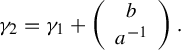 $$ \begin{align*}\gamma_2 = \gamma_1 + \left( \begin{array}{ c c } b \\ a^{-1} \end{array} \right).\end{align*} $$
Similarly,
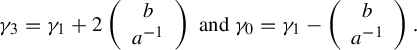 $$ \begin{align*}\gamma_3 = \gamma_1 + 2\left( \begin{array}{ c c } b \\ a^{-1} \end{array} \right)\text{ and } \gamma_0 = \gamma_1 - \left( \begin{array}{ c c } b \\ a^{-1} \end{array} \right).\end{align*} $$
Of course, if we add the basis vector
 $(b, a^{-1})^T$
too many times, the horizontal will become larger than 1 and hence we will cease to have a candidate. This is amended by subtracting the other basis vector
$(b, a^{-1})^T$
too many times, the horizontal will become larger than 1 and hence we will cease to have a candidate. This is amended by subtracting the other basis vector
 $(a,0)^T$
, but this makes the slope larger since we are decreasing the horizontal. In other words, the only candidates
$(a,0)^T$
, but this makes the slope larger since we are decreasing the horizontal. In other words, the only candidates
 $\gamma _n$
in which we are interested are those to which we can add the basis vector
$\gamma _n$
in which we are interested are those to which we can add the basis vector
 $(b, a^{-1})^T$
so that they still have a horizontal less than or equal to
$(b, a^{-1})^T$
so that they still have a horizontal less than or equal to
 $1$
. In particular, this is a finite list. We can then obtain the candidate with minimum slope by observing how adding the basis vector
$1$
. In particular, this is a finite list. We can then obtain the candidate with minimum slope by observing how adding the basis vector
 $(b, a^{-1})^T$
changes the slope compared with
$(b, a^{-1})^T$
changes the slope compared with
 $\gamma _1$
. Now notice that
$\gamma _1$
. Now notice that
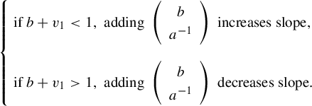 $$ \begin{align*}\begin{cases} \text{ if } b+v_1<1, \text{ adding } \left( \begin{array}{ c c } b \\ a^{-1} \end{array} \right) \text{ increases slope, }\\ \text{ if } b+v_1>1,\text{ adding } \left( \begin{array}{ c c } b \\ a^{-1} \end{array} \right) \text{ decreases slope. }\\ \end{cases}\end{align*} $$
We conclude the following.
-
(1) If
$b+v_1<1$
, then the minimum of the slopes is
$\min \{\text {slope }(\gamma _0), \text {slope } (\gamma _1)\}$
. A direct calculation shows that the minimum of these two is
$\text {slope }(\gamma _0) = v_2/v_1$
. -
(2) If
$b+v_1>1$
, then the minimum of the slopes is slope
$(\gamma _j)$
, where j is the maximum number of times we can add
$(\begin {smallmatrix} b \\ a^{-1} \end {smallmatrix})$
to
$\gamma _1$
so that the horizontal of
$\gamma _j$
is smaller than 1. We compute this value of j: this is the largest number so that
$$ \begin{align*}\text{ horizontal }(\gamma_j) = jb+v_1 -a \le 1<(j+1)b+v_1 -a \kern1.5pt{\iff}\kern1.5pt j=\bigg\lfloor\kern-1.5pt \frac{a+1-v_1}{b}\kern-1.5pt\bigg\rfloor.\end{align*} $$


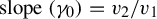


Hence, for an element
 $\omega \in \mathcal W _{\mathrm{sl}}$
, with
$\omega \in \mathcal W _{\mathrm{sl}}$
, with
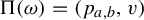 $\Pi (\omega )=(p_{a,b},v)$
, to return to
$\Pi (\omega )=(p_{a,b},v)$
, to return to
 $\mathcal W _{\mathrm{sa}}$
under the horocycle flow, it needs to travel
$\mathcal W _{\mathrm{sa}}$
under the horocycle flow, it needs to travel
 $\rho $
units of time, where
$\rho $
units of time, where
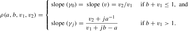 $$ \begin{align*}\rho(a,b,v_1,v_2) = \begin{cases} \text{ slope }(\gamma_0) = \text{ slope }(v) = v_2/v_1 &\text{ if } b+v_1 \le 1, \text{ and }\\ \text{ slope }(\gamma_j) = \dfrac{v_2 + ja^{-1}}{v_1+jb-a} &\text{ if } b+v_1> 1. \end{cases}\\[-44pt]\end{align*} $$
Now we give the proof of the return time to
 $\mathcal W$
under horocycle flow.
$\mathcal W$
under horocycle flow.
Proof Proof of Theorem 3.11
Step 1: Computing time from
 $W_ {sa}/\mathcal W_{\mathrm{sl}}$
to
$W_ {sa}/\mathcal W_{\mathrm{sl}}$
to
 $W_{\mathrm{sa}}/\mathcal W_{\mathrm{sl}}$
. We implement the first part of the strategy outlined at the beginning of this section and compute how much time is needed for an element in
$W_{\mathrm{sa}}/\mathcal W_{\mathrm{sl}}$
. We implement the first part of the strategy outlined at the beginning of this section and compute how much time is needed for an element in
 $\mathcal W$
to return to either
$\mathcal W$
to return to either
 $\mathcal W_{\mathrm{sl}}$
or
$\mathcal W_{\mathrm{sl}}$
or
 $\mathcal W_{\mathrm{sa}}$
.
$\mathcal W_{\mathrm{sa}}$
.
(1) Time from
 $\mathcal W _{\mathrm{sa}}$
to
$\mathcal W _{\mathrm{sa}}$
to
 $\mathcal W _{\mathrm{sa}}$
: Suppose that
$\mathcal W _{\mathrm{sa}}$
: Suppose that
 $\omega \in \mathcal W _{\mathrm{sa}}$
so that
$\omega \in \mathcal W _{\mathrm{sa}}$
so that
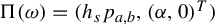 $\Pi (\omega )=(h_sp_{a,b},({\alpha },0)^T)$
for
$\Pi (\omega )=(h_sp_{a,b},({\alpha },0)^T)$
for
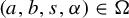 $(a,b,s,{\alpha })\in \Omega $
. Consequently, the return time to
$(a,b,s,{\alpha })\in \Omega $
. Consequently, the return time to
 $\mathcal W _{\mathrm{sa}} \subset \mathcal W$
is exactly the return time from the previous section on affine lattices. Namely, the return time is
$\mathcal W _{\mathrm{sa}} \subset \mathcal W$
is exactly the return time from the previous section on affine lattices. Namely, the return time is
 $R(a,b,s,{\alpha })$
.
$R(a,b,s,{\alpha })$
.
(2) Time from
 $\mathcal W _{\mathrm{sa}}$
to
$\mathcal W _{\mathrm{sa}}$
to
 $\mathcal W _{\mathrm{sl}}$
: Suppose that
$\mathcal W _{\mathrm{sl}}$
: Suppose that
 $\omega \in \mathcal W _{\mathrm{sa}}$
so that
$\omega \in \mathcal W _{\mathrm{sa}}$
so that
 $\Pi (\omega )=(h_sp_{a,b},({\alpha },0)^T)$
for
$\Pi (\omega )=(h_sp_{a,b},({\alpha },0)^T)$
for
 $(a,b,s,{\alpha })\in \Omega $
. Consequently, under the horocycle flow, the next time we get a short vector in the lattice part is when the lattice part contains a short vector. Hence, the return time to
$(a,b,s,{\alpha })\in \Omega $
. Consequently, under the horocycle flow, the next time we get a short vector in the lattice part is when the lattice part contains a short vector. Hence, the return time to
 $\mathcal W _{\mathrm{sl}}\subset \mathcal W$
is
$\mathcal W _{\mathrm{sl}}\subset \mathcal W$
is
 $(ab)^{-1}-s$
from the results of [Reference Athreya and Cheung5].
$(ab)^{-1}-s$
from the results of [Reference Athreya and Cheung5].
(3) Time from
 $\mathcal W _{\mathrm{sl}}$
to
$\mathcal W _{\mathrm{sl}}$
to
 $\mathcal W _{\mathrm{sl}}$
: Suppose that
$\mathcal W _{\mathrm{sl}}$
: Suppose that
 $\omega \in \mathcal W _{\mathrm{sl}}$
so that
$\omega \in \mathcal W _{\mathrm{sl}}$
so that
 $\Pi (\omega ) =(p_{a,b},v)$
for some
$\Pi (\omega ) =(p_{a,b},v)$
for some
 $(a,b)\in \Delta .$
Thus, under the horocycle flow, the next time we get a short vector in the lattice part is the return time obtained from [Reference Athreya and Cheung5]. Hence, the return time to
$(a,b)\in \Delta .$
Thus, under the horocycle flow, the next time we get a short vector in the lattice part is the return time obtained from [Reference Athreya and Cheung5]. Hence, the return time to
 $\mathcal W _{\mathrm{sl}}\subset \mathcal W$
is
$\mathcal W _{\mathrm{sl}}\subset \mathcal W$
is
 $(ab)^{-1}$
from the results of [Reference Athreya and Cheung5].
$(ab)^{-1}$
from the results of [Reference Athreya and Cheung5].
(4) Time from
 $\mathcal W _{\mathrm{sl}}$
to
$\mathcal W _{\mathrm{sl}}$
to
 $\mathcal W _{\mathrm{sa}}$
: The only difficult return time
$\mathcal W _{\mathrm{sa}}$
: The only difficult return time
 $\rho (a,b,v_1,v_2)$
to compute is for an element
$\rho (a,b,v_1,v_2)$
to compute is for an element
 $\omega \in \mathcal W _{\mathrm{sl}}$
to return to
$\omega \in \mathcal W _{\mathrm{sl}}$
to return to
 $\mathcal W _{\mathrm{sa}}$
. This was computed in the previous lemma to be
$\mathcal W _{\mathrm{sa}}$
. This was computed in the previous lemma to be
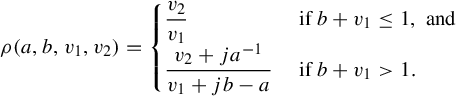 $$ \begin{align*}\rho(a,b,v_1,v_2) = \begin{cases} \dfrac{v_2}{v_1} &\text{ if } b+v_1 \le 1, \text{ and }\\ \dfrac{v_2 + ja^{-1}}{v_1+jb-a} &\text{ if } b+v_1> 1.\\ \end{cases}\end{align*} $$
We collect the times collected above now to deduce that for
 $\omega \in \mathcal W$
, the return time u to
$\omega \in \mathcal W$
, the return time u to
 $\mathcal W$
under the horocycle flow is given by the following two cases.
$\mathcal W$
under the horocycle flow is given by the following two cases.
Case 1:
 $\omega \in \mathcal W_{\mathrm{sl}}$
. For
$\omega \in \mathcal W_{\mathrm{sl}}$
. For
 $\omega \in \mathcal W_{\mathrm{sl}}$
, the return time is
$\omega \in \mathcal W_{\mathrm{sl}}$
, the return time is
 $$ \begin{align*}u = \min\{(ab)^{-1}, \rho(a,b,v_1,v_2)\}\end{align*} $$
where
 $\rho $
is the minimum time it takes for an affine lattice
$\rho $
is the minimum time it takes for an affine lattice
 $(p_{a,b},v)$
to have a short affine vector in the affine piece.
$(p_{a,b},v)$
to have a short affine vector in the affine piece.
Case 2:
 $\omega \in \mathcal W_{\mathrm{sa}}$
. For
$\omega \in \mathcal W_{\mathrm{sa}}$
. For
 $\omega \in \mathcal W_{\mathrm{sa}}$
, the return time is
$\omega \in \mathcal W_{\mathrm{sa}}$
, the return time is
 $$ \begin{align*}u = \min \{(ab)^{-1}-s,R(a,b,s,{\alpha})\}\end{align*} $$
where R is the return map for affine lattices.
Step 2: Computing the minimum. We now implement the second step of the strategy and compute the minimums of the times calculated from step 1. We have two cases given by the partition of
 $\mathcal W$
.
$\mathcal W$
.
Case 1:
 $\omega \in \mathcal W_{\mathrm{sl}}$
. For
$\omega \in \mathcal W_{\mathrm{sl}}$
. For
 $\omega \in \mathcal W_{\mathrm{sl}}$
the return time is
$\omega \in \mathcal W_{\mathrm{sl}}$
the return time is
 $$ \begin{align*}u = \min\{(ab)^{-1}, \rho(a,b,v_1,v_2)\}\end{align*} $$
where we have
 $\Pi (\omega )=(p_{a,b},v)$
for some
$\Pi (\omega )=(p_{a,b},v)$
for some
 $(a,b)\in \Delta $
and
$(a,b)\in \Delta $
and
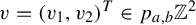 $v=(v_1,v_2)^T\in p_{a,b}{\mathbb {Z}}^2$
. The return time is
$v=(v_1,v_2)^T\in p_{a,b}{\mathbb {Z}}^2$
. The return time is
 $$ \begin{align*}u = \begin{cases} \min \{(ab)^{-1},v_2/v_1\} &\text{ if } b+v_1 \le 1, \text{ and }\\ \min\bigg\{ (ab)^{-1}, \dfrac{v_2 + ja^{-1}}{v_1+jb-a}\bigg\} &\text{ if } b+v_1> 1.\\ \end{cases}\end{align*} $$
By our choice of v as the representative lying in the standard fundamental domain of
 ${\mathbb {R}}^2/p_{a,b}{\mathbb {Z}}^2$
spanned by the columns of
${\mathbb {R}}^2/p_{a,b}{\mathbb {Z}}^2$
spanned by the columns of
 $p_{a,b}$
, we have
$p_{a,b}$
, we have
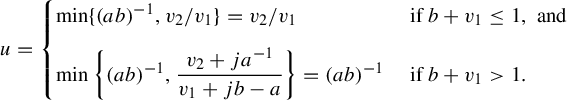 $$ \begin{align*}u = \begin{cases} \min \{(ab)^{-1},v_2/v_1\} = v_2/v_1 &\text{ if } b+v_1 \le 1, \text{ and }\\ \min\bigg\{ (ab)^{-1}, \dfrac{v_2 + ja^{-1}}{v_1+jb-a}\bigg\} = (ab)^{-1} &\text{ if } b+v_1> 1.\\ \end{cases}\end{align*} $$
Case 2:
 $\omega \in \mathcal W_{\mathrm{sa}}$
. For
$\omega \in \mathcal W_{\mathrm{sa}}$
. For
 $\omega \in \mathcal W_{\mathrm{sa}}$
, the return time is
$\omega \in \mathcal W_{\mathrm{sa}}$
, the return time is
 $$ \begin{align*}u = \min \{(ab)^{-1}-s,R(a,b,s,{\alpha})\}\end{align*} $$
where R is the return map for affine lattices and
 $(a,b,s,{\alpha })\in \Omega $
. Recall the map is defined piecewise as
$(a,b,s,{\alpha })\in \Omega $
. Recall the map is defined piecewise as
 $$ \begin{align*}R(a,b,s,{\alpha}) = \begin{cases} \dfrac{sa}{{\alpha}-a} &\text{ if } (a,b,s,{\alpha})\in\Omega_1,\\ \dfrac{j(a^{-1}-sb)+sa}{{\alpha}-a+jb} &\text{ if } (a,b,s,{\alpha})\in\Omega_2,\\ \dfrac{a^{-1}-sb}{b+{\alpha}} &\text{ if } (a,b,s,{\alpha})\in\Omega_3,\\ \dfrac{j(a^{-1}-sb)}{{\alpha}-a+jb} &\text{ if } (a,b,s,{\alpha})\in\Omega_4. \end{cases}\end{align*} $$
where
 $j=\lfloor ({1+a-\alpha })/{b}\rfloor $
. We now compute the return time
$j=\lfloor ({1+a-\alpha })/{b}\rfloor $
. We now compute the return time
 $$ \begin{align*}u = \min \{(ab)^{-1}-s,R(a,b,s,{\alpha})\}.\end{align*} $$
-
(1) If
$(a,b,s,{\alpha })\in \Omega _1$
, then
$$ \begin{align*}u=\frac{sa}{{\alpha}-a}\end{align*} $$
because
and this inequality is one of the defining inequalities of
$$ \begin{align*}\frac{sa}{{\alpha}-a}<(ab)^{-1}-s\!\iff s<\frac{{\alpha}-a}{ab{\alpha}}\end{align*} $$
$\Omega _1.$
-
(2) If
$(a,b,s,{\alpha })\in \Omega _2$
, then because
$$ \begin{align*}u=(ab)^{-1}-s\end{align*} $$
and this inequality is one of the defining inequalities of
$$ \begin{align*}(ab)^{-1}-s<\frac{j(a^{-1}-sb)+sa}{{\alpha}-a+jb}\iff s>\frac{{\alpha}-a}{ab{\alpha}}\end{align*} $$
$\Omega _2.$
-
(3) If
$(a,b,s,{\alpha })\in \Omega _3$
, then because
$$ \begin{align*}u=\frac{a^{-1}-sb}{b+{\alpha}}\end{align*} $$
and this inequality is one of the defining inequalities of
$$ \begin{align*}\frac{a^{-1}-sb}{b+{\alpha}}<(ab)^{-1}-s\!\iff s<\frac{1}{ab}\end{align*} $$
$\Omega .$
-
(4) If
$(a,b,s,{\alpha })\in \Omega _4$
, then because
$$ \begin{align*}u=(ab)^{-1}-s\end{align*} $$
and this inequality is one of the defining inequalities of
$$ \begin{align*}(ab)^{-1}-s< \frac{j(a^{-1}-sb)}{{\alpha}-a+jb}\iff s<\frac{1}{ab}\end{align*} $$
$\Omega .$


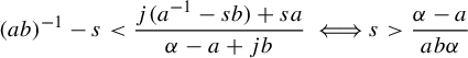


4 Invariant measures and gap distributions
Here, we prove the existence of a density function for the slope gap question for twice-marked tori and for doubled slit tori. We will classify measures on the transversal
 $\Omega $
and show various properties of the cumulative distribution function of the gaps such as support at zero and the decay rate. We will also consider an invariant measure on the transversal
$\Omega $
and show various properties of the cumulative distribution function of the gaps such as support at zero and the decay rate. We will also consider an invariant measure on the transversal
 $\mathcal W$
.
$\mathcal W$
.
4.1 Invariant measures on
$\Omega $

In this section, we review some Ratner theory and use it classify invariant measures on
 $\Omega $
.
$\Omega $
.
4.1.1 Ratner theory for
$AX_2$

In the early 1990s, Marina Ratner published a series of influential works [Reference Ratner22–Reference Ratner24] that gave a mostly complete understanding of ergodic probability measures for unipotent dynamical systems on homogenous spaces. We briefly review her work in the context of horocycle flow on
 $AX_2$
. Our exposition borrows ideas from [Reference Arbieto, Matheus and Moreira1, Reference Eskin11, Reference Strömbergsson27].
$AX_2$
. Our exposition borrows ideas from [Reference Arbieto, Matheus and Moreira1, Reference Eskin11, Reference Strömbergsson27].
Consider the vertical translation
 $V_\beta :AX_2\to AX_2$
 $$ \begin{align*}V_\beta(g,v) = \left(g,v + \left( \begin{array}{ c c } 0 \\ \beta \end{array} \right)\right)\end{align*} $$
for some
 $\beta \in {\mathbb {R}}$
. Notice that this flow always commutes with
$\beta \in {\mathbb {R}}$
. Notice that this flow always commutes with
 $h_s$
. Hence, if
$h_s$
. Hence, if
 $\mu $
is an ergodic probability measure invariant under horocycle flow, then so is the measure obtained by precomposing with
$\mu $
is an ergodic probability measure invariant under horocycle flow, then so is the measure obtained by precomposing with
 $V_\beta $
. This makes it interesting to consider the vertical translation if one is interested in measures invariant under the horocycle flow.
$V_\beta $
. This makes it interesting to consider the vertical translation if one is interested in measures invariant under the horocycle flow.
By disintegrating, any measure
 $\,d\mu (g,v)$
on
$\,d\mu (g,v)$
on
 $AX_2$
can be decomposed into the measure
$AX_2$
can be decomposed into the measure
 $$ \begin{align*}\,d\mu (g,v) =\,d\lambda_g(v) \,d \nu (g),\end{align*} $$
where
 $\,d \nu (g)$
is a measure on the lattice part and
$\,d \nu (g)$
is a measure on the lattice part and
 $\,d\lambda _g(v)$
is a measure on the fiber. Notice that the vertical translation only acts on the fiber piece of an affine lattice
$\,d\lambda _g(v)$
is a measure on the fiber. Notice that the vertical translation only acts on the fiber piece of an affine lattice
 $(g,v)$
. (That is, it acts on the torus
$(g,v)$
. (That is, it acts on the torus
 ${\mathbb {R}}^2/g{\mathbb {Z}}^2.$
) We can use previous results of [Reference Furstenberg14] (in the cocompact case) and [Reference Dani8] (in the general lattice case) to understand the possibilities for
${\mathbb {R}}^2/g{\mathbb {Z}}^2.$
) We can use previous results of [Reference Furstenberg14] (in the cocompact case) and [Reference Dani8] (in the general lattice case) to understand the possibilities for
 $\nu (g)$
. These results show that either
$\nu (g)$
. These results show that either
 $\nu $
is a Haar measure on
$\nu $
is a Haar measure on
 $X_2$
or supports a periodic measure. Given these two possible measures on the lattice part, we can then try to understand how vertical translation acts on the fiber
$X_2$
or supports a periodic measure. Given these two possible measures on the lattice part, we can then try to understand how vertical translation acts on the fiber
 ${\mathbb {R}}^2/g{\mathbb {Z}}^2$
to gain a complete understanding of the possibilities for
${\mathbb {R}}^2/g{\mathbb {Z}}^2$
to gain a complete understanding of the possibilities for
 $\mu $
. This is carried out in [Reference Eskin11]. Before being more precise, we make some definitions.
$\mu $
. This is carried out in [Reference Eskin11]. Before being more precise, we make some definitions.
The denominator of an affine lattice
 $(g,v)$
is the minimal
$(g,v)$
is the minimal
 $d>0$
so that
$d>0$
so that
 $v\in d^{-1}g{\mathbb {Z}}^2$
whenever this is defined. We denote the denominator by
$v\in d^{-1}g{\mathbb {Z}}^2$
whenever this is defined. We denote the denominator by
 $d(g,v).$
Let
$d(g,v).$
Let
 $X[q]$
denote the set of affine lattices with denominator
$X[q]$
denote the set of affine lattices with denominator
 $q>0.$
That is,
$q>0.$
That is,
 $$ \begin{align*}X[q]=\{ (g,v)\in AX_2: d(g,v)=q \}.\end{align*} $$
In the literature, this is also referred to as the set of torsion affine lattices since the vector v for any
 $(g,v)\in X[q]$
is a torsion point under the group structure of
$(g,v)\in X[q]$
is a torsion point under the group structure of
 ${\mathbb {C}}/g{\mathbb {Z}}^2$
. The set of torsion affine lattices forms an
${\mathbb {C}}/g{\mathbb {Z}}^2$
. The set of torsion affine lattices forms an
 ${\textrm {SL}}_2({\mathbb {R}})$
-invariant subset of
${\textrm {SL}}_2({\mathbb {R}})$
-invariant subset of
 $AX_2$
of dimension 3. In particular, it is a homogenous space and can be identified as the quotient of
$AX_2$
of dimension 3. In particular, it is a homogenous space and can be identified as the quotient of
 ${\textrm {SL}}_2({\mathbb {R}})$
by
${\textrm {SL}}_2({\mathbb {R}})$
by
 $\Gamma (q)$
, where
$\Gamma (q)$
, where
 $\Gamma (q)$
is the congruence subgroup
$\Gamma (q)$
is the congruence subgroup
 $$ \begin{align*}\Gamma(q)=\{\gamma \in {\textrm{SL}}_2({\mathbb{Z}}):\gamma \equiv {\textrm{Id}}\!\!\! \mod\!q\}.\end{align*} $$
Explicitly, this identification is given by the map
 $$ \begin{align*}g({\mathbb{Z}}^2 + w)\mapsto g\Gamma(q),\end{align*} $$
where w is any vector with denominator q.
To get an idea of the properties of these types of affine lattices, notice that
 $X[1]$
is just the space of lattices. Also notice that
$X[1]$
is just the space of lattices. Also notice that
 $({\textrm {Id}}, (\begin {smallmatrix} 1/2 \\ 1/2 \end {smallmatrix}))$
is
$({\textrm {Id}}, (\begin {smallmatrix} 1/2 \\ 1/2 \end {smallmatrix}))$
is
 $X[2]$
, but not in
$X[2]$
, but not in
 $X[4]$
by our minimality condition on the denominator.
$X[4]$
by our minimality condition on the denominator.
Thinking about torsion affine lattices as twice-marked tori, we see that torsion twice-marked tori are lattices surfaces. This explains our assumption that restricts to affine lattices with
 $v\notin g{\mathbb {Q}}^2$
. In fact, we have
$v\notin g{\mathbb {Q}}^2$
. In fact, we have
 $(g,v)$
is a lattice surface if and only if
$(g,v)$
is a lattice surface if and only if
 $v\in g{\mathbb {Q}}^2$
, see the work of Schmoll [Reference Schmoll25] for proof of this.
$v\in g{\mathbb {Q}}^2$
, see the work of Schmoll [Reference Schmoll25] for proof of this.
We now state Ratner’s measure classification for horocycle flow on
 $AX_2$
.
$AX_2$
.
Theorem 4.1. If
 $\mu $
is an
$\mu $
is an
 $h_u$
-invariant ergodic probability measure, then
$h_u$
-invariant ergodic probability measure, then
 $\mu $
is one of the following:
$\mu $
is one of the following:
-
(1)
$\mu =m_{AX_2}$
, the Haar measure on
$AX_2$
; -
(2)
$\mu $
is a torsion measure, that is, there is
$q>0$
so that the support of
$\mu $
is contained in the set of torsion affine lattices
$X[q]$
; -
(3) there is
$a>0$
and
$ 0\le {\alpha }<a^{-1}$
so that the support of
$\mu $
is
$$ \begin{align*}&\text{Per}(a,{\alpha})\\&\quad:= \left\{h_sV_\beta \left(g_{\log(a)}, \left( \begin{array}{ c c } {\alpha} \\ 0 \end{array} \right)\right) = \left(h_sg_{\log(a)}, \left( \begin{array}{ c c } {\alpha} \\ \beta \end{array} \right)\right):s\in[0,a^2),\beta\in[0,a)\right\};\end{align*} $$
-
(4)
$\mu $
is supported on a
$h_u$
-periodic orbit.


The first two measure above are those whose lattice measure is a Haar measure on
 $X_2$
, while the remaining two are those for which the lattice measure is supported on a
$X_2$
, while the remaining two are those for which the lattice measure is supported on a
 $h_u$
-periodic orbit.
$h_u$
-periodic orbit.
Lastly, we observe that any measure in the list above can be precomposed by a vertical translation
 $V_\beta $
to produce more ergodic probability measures. We will mainly concern ourselves with the above list.
$V_\beta $
to produce more ergodic probability measures. We will mainly concern ourselves with the above list.
4.1.2 Invariant measures for
$\Omega $

To classify ergodic probability measures invariant under the return map on the transversal
 $\Omega $
, we use Ratner’s theorem, which classifies ergodic probability measures for unipotent dynamical systems on homogenous spaces. Since we have a transversal, then there is a bridge between measures on
$\Omega $
, we use Ratner’s theorem, which classifies ergodic probability measures for unipotent dynamical systems on homogenous spaces. Since we have a transversal, then there is a bridge between measures on
 $(AX_2,h_s)$
and measures on
$(AX_2,h_s)$
and measures on
 $(\Omega ,T)$
. While this bridge is well known by now, the interested reader can find details in [Reference Athreya and Cheung5].
$(\Omega ,T)$
. While this bridge is well known by now, the interested reader can find details in [Reference Athreya and Cheung5].
As a corollary to Ratner’s theorem, we can classify T-invariant measures on the transversal
 $\Omega $
by disintegration.
$\Omega $
by disintegration.
Theorem 4.2. If
 $\nu $
is a T-invariant ergodic probability measure, then:
$\nu $
is a T-invariant ergodic probability measure, then:
-
(1)
$\nu $
is induced by the Haar measure on
$AX_2$
, that is,
$d \nu = 2\,ds\,db\,da\,d{\alpha } $
; -
(2)
$\nu $
is induced by a torsion measure on
$AX_2$
and is given by the two-dimensional Lebesgue measure on a finite number of triangles; -
(3)
$\nu $
is supported on for some
$$ \begin{align*}\Omega\cap \text{Per}(a,{\alpha})= \left\{ \left(h_sg_{\log(a)}, \left( \begin{array}{ c c } {\alpha} \\ 0 \end{array} \right)\right):s\in[0,a^2)\right\}\end{align*} $$
$a>0$
and
$ 0\le {\alpha }<\min \{a^{-1},1\}$
;
-
(4)
$\nu $
is supported on a T-periodic orbit.


Proof By our discussion about disintegration in the last section, it is clear that the disintegration of the Haar measure on
 $AX_2$
is given by the product of the two-dimensional Lebesgue measure on the torus
$AX_2$
is given by the product of the two-dimensional Lebesgue measure on the torus
 ${\mathbb {R}}^2/g{\mathbb {Z}}^2$
and the three-dimensional Haar measure on
${\mathbb {R}}^2/g{\mathbb {Z}}^2$
and the three-dimensional Haar measure on
 $X_2.$
This measure is
$X_2.$
This measure is
 ${\textrm {SL}}_2({\mathbb {R}})$
-invariant and hence horocycle invariant. On
${\textrm {SL}}_2({\mathbb {R}})$
-invariant and hence horocycle invariant. On
 $\Omega $
, we must consider only those affine lattices with a short horizontal vector so that the disintegration of the Haar measure on
$\Omega $
, we must consider only those affine lattices with a short horizontal vector so that the disintegration of the Haar measure on
 $\Omega $
will be
$\Omega $
will be
 $$ \begin{align*}\,dm_{\Omega} = 2\,ds\,db\,da\,d{\alpha} .\end{align*} $$
Now suppose that
 $\nu $
is a T-invariant ergodic probability measure on
$\nu $
is a T-invariant ergodic probability measure on
 $\Omega $
, different than
$\Omega $
, different than
 $m_\Omega $
. Consider
$m_\Omega $
. Consider
 $\, d\nu \, du$
on
$\, d\nu \, du$
on
 $AX_2$
. By Ratner’s theorem, we know the support of this measure on
$AX_2$
. By Ratner’s theorem, we know the support of this measure on
 $AX_2$
can only be three-, two-, or one-dimensional.
$AX_2$
can only be three-, two-, or one-dimensional.
In case it is three-dimensional, then it must be supported on
 $X[q]$
for some
$X[q]$
for some
 $q>0$
. In particular, this means that we are in the territory of lattice surfaces and the work of Uyanik and Work [Reference Uyanik and Work29] applies. Their work shows that the transversal of short horizontal saddle connections
$q>0$
. In particular, this means that we are in the territory of lattice surfaces and the work of Uyanik and Work [Reference Uyanik and Work29] applies. Their work shows that the transversal of short horizontal saddle connections
 $\Omega \cap X[q]$
is given by k triangles, where k is the number of cusps of
$\Omega \cap X[q]$
is given by k triangles, where k is the number of cusps of
 $X[q]$
thought of as
$X[q]$
thought of as
 ${\textrm {SL}}_2({\mathbb {R}})/\Gamma (q)$
. In particular, the T-invariant ergodic probability measure is given by the Lebesgue measure on these triangles. We refer the interested reader to their work for more details.
${\textrm {SL}}_2({\mathbb {R}})/\Gamma (q)$
. In particular, the T-invariant ergodic probability measure is given by the Lebesgue measure on these triangles. We refer the interested reader to their work for more details.
In case
 $d\nu \, du$
is two-dimensional, then it is supported on
$d\nu \, du$
is two-dimensional, then it is supported on
 $\text {Per}(a,{\alpha })$
for some
$\text {Per}(a,{\alpha })$
for some
 $a>0$
and
$a>0$
and
 $ 0\le {\alpha }<\min \{a^{-1},1\}$
, that is, those affine lattices for which the lattice part is periodic and the affine piece has an arbitrary vertical component. Hence,
$ 0\le {\alpha }<\min \{a^{-1},1\}$
, that is, those affine lattices for which the lattice part is periodic and the affine piece has an arbitrary vertical component. Hence,
 $\,d\nu $
is supported on
$\,d\nu $
is supported on
 $$ \begin{align*}\Omega\cap \text{Per}(a,{\alpha})= \left\{ \left(h_sg_{\log(a)}, \left( \begin{array}{ c c } {\alpha} \\ 0 \end{array} \right)\right):s\in[0,a^2)\right\}.\end{align*} $$
Lastly, if
 $d\nu \, du$
is one-dimensional, then on
$d\nu \, du$
is one-dimensional, then on
 $\Omega $
it becomes zero-dimensional. This simply means that it is supported on a periodic orbit for T.
$\Omega $
it becomes zero-dimensional. This simply means that it is supported on a periodic orbit for T.
We continue to refer to the measure
 $m_\Omega $
as the Haar measure on
$m_\Omega $
as the Haar measure on
 $\Omega $
and we use
$\Omega $
and we use
 $m_q$
to denote a torsion measure on the transversal. We obtain the following.
$m_q$
to denote a torsion measure on the transversal. We obtain the following.
Theorem 4.3. The measure
 $dm_{\Omega } = 2\,ds\,db\,da\,d{\alpha } $
is a unique T-invariant ergodic probability measure on
$dm_{\Omega } = 2\,ds\,db\,da\,d{\alpha } $
is a unique T-invariant ergodic probability measure on
 $\Omega $
that is absolutely continuous with respect to the Lebesgue measure. Hence, for almost every
$\Omega $
that is absolutely continuous with respect to the Lebesgue measure. Hence, for almost every
 $m_\Omega $
point
$m_\Omega $
point
 $(a,b,s,{\alpha })$
and every
$(a,b,s,{\alpha })$
and every
 $f\in L^1(\Omega )$
,
$f\in L^1(\Omega )$
,
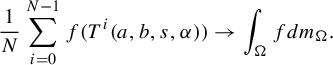 $$ \begin{align*}\frac{1}{N}\sum_{i=0} ^{N-1}f(T^i(a,b,s,{\alpha}))\to \int_\Omega f dm_{\Omega}.\end{align*} $$
In coordinates
 $(a,b,s,{\alpha })$
, integrating with respect to
$(a,b,s,{\alpha })$
, integrating with respect to
 $dm_{\Omega }$
takes the form
$dm_{\Omega }$
takes the form
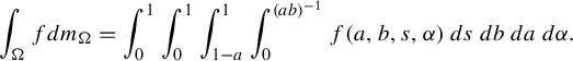 $$ \begin{align*}\int _\Omega f dm_\Omega = \int _{0} ^1 \int_{0} ^1 \int_{1-a} ^ 1 \int _{0} ^{(ab)^{-1}} f(a,b,s,{\alpha})\,ds\,db\,da\,d{\alpha}.\end{align*} $$
4.2 An invariant measure on
$\mathcal W$

Recall that
 $\mathcal H(0,0)=AX_2$
is a homogenous space so that it comes equipped with a Haar measure
$\mathcal H(0,0)=AX_2$
is a homogenous space so that it comes equipped with a Haar measure
 $m_{AX_2}$
. Since
$m_{AX_2}$
. Since
 ${\mathcal {W}}$
is a four-fold cover of
${\mathcal {W}}$
is a four-fold cover of
 $AX_2$
, we can endow it with a natural measure that is four copies of
$AX_2$
, we can endow it with a natural measure that is four copies of
 $m_{AX_2}$
. Denote this measure by
$m_{AX_2}$
. Denote this measure by
 $m_{{\mathcal {E}}}.$
This measure is
$m_{{\mathcal {E}}}.$
This measure is
 ${\textrm {SL}}_2({\mathbb {R}})$
-invariant and finite. In particular, this measure is also invariant under the horocycle flow.
${\textrm {SL}}_2({\mathbb {R}})$
-invariant and finite. In particular, this measure is also invariant under the horocycle flow.
There is a correspondence of measures invariant under a flow and measures invariant under the first return map of that flow to a transversal. Specializing to our situation, there is an induced measure on our transversal
 $\mathcal W$
, which we denote by
$\mathcal W$
, which we denote by
 $m_{\mathcal W}$
, that is invariant under the first return map.
$m_{\mathcal W}$
, that is invariant under the first return map.
It can be written as the sum of a Lebesgue measure on
 $W_{\mathrm{sl}}$
and
$W_{\mathrm{sl}}$
and
 $W_{\mathrm{sa}}$
, which we denote as
$W_{\mathrm{sa}}$
, which we denote as
 $m_{\mathrm{sa}}$
and
$m_{\mathrm{sa}}$
and
 $m_{\mathrm{sl}}$
. Explicitly, on
$m_{\mathrm{sl}}$
. Explicitly, on
 ${\mathcal {W}}_{\mathrm{sa}}$
, we have
${\mathcal {W}}_{\mathrm{sa}}$
, we have
 $\Pi (\omega )= \Lambda _{(a,b,s,{\alpha })}\in \Omega $
and so for
$\Pi (\omega )= \Lambda _{(a,b,s,{\alpha })}\in \Omega $
and so for
 $f\in L^1({\mathcal {W}}_{\mathrm{sa}})$
, we have
$f\in L^1({\mathcal {W}}_{\mathrm{sa}})$
, we have
 $$ \begin{align*}\int_{{\mathcal{W}}_{\mathrm{sa}}} f \,dm_{\mathrm{sa}}= 4\int_{\Omega} f(a,b,s,{\alpha})\,ds \,db \,da \,d{\alpha},\end{align*} $$
where the 4 reflects the fact that the
 $\Pi :\mathcal E\to \mathcal H(0,0)=AX_2$
is a four-to-one map. Similarly, on
$\Pi :\mathcal E\to \mathcal H(0,0)=AX_2$
is a four-to-one map. Similarly, on
 ${\mathcal {W}}_{\mathrm{sl}}$
, we have
${\mathcal {W}}_{\mathrm{sl}}$
, we have
 $\Pi (\omega )= (p_{a,b},v)$
, where
$\Pi (\omega )= (p_{a,b},v)$
, where
 $(a,b)\in \Delta $
and
$(a,b)\in \Delta $
and
 $v\in {\mathbb {R}}^2/p_{a,b}{\mathbb {Z}}^2$
, and so for
$v\in {\mathbb {R}}^2/p_{a,b}{\mathbb {Z}}^2$
, and so for
 $f\in L^1({\mathcal {W}}_{\mathrm{sl}})$
, we have
$f\in L^1({\mathcal {W}}_{\mathrm{sl}})$
, we have
 $$ \begin{align*}\int_{{\mathcal{W}}_{\mathrm{sl}}} f \,dm_{\mathrm{sl}}= 4 \iint\limits_{(a,b)\in\Delta}\int_{v\in {\mathbb{R}}^2/p_{a,b}{\mathbb{Z}}^2} f(a,b,v)\,dv \,db \,da.\end{align*} $$
Thus, the flat measure on
 ${\mathcal {W}}$
is given by the sum,
${\mathcal {W}}$
is given by the sum,
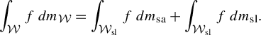 $$ \begin{align*}\int _{\mathcal{W}} f \,dm_{{\mathcal{W}}} = \int_{{\mathcal{W}}_{\mathrm{sl}}} f \,dm_{\mathrm{sa}} +\int_{{\mathcal{W}}_{\mathrm{sl}}} f \,dm_{\mathrm{sl}}.\end{align*} $$
4.3 Gap distribution results
In this section, we prove the existence of the slope gap limit for twice-marked tori and doubled slit tori and state various properties about their distribution and density functions.
Proof Proof of Theorem 2.2
We prove that the slope gap limit in Theorem 2.2 of twice-marked tori exists. Recall from (6), we have
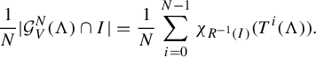 $$ \begin{align*}\frac{1}{N}|\mathcal G^N _V(\Lambda)\cap I|=\frac{1}{N}\sum_{i=0} ^{N-1}\chi_{ R^{-1}(I)}(T^i(\Lambda)).\end{align*} $$
Now suppose that
 $\Lambda $
is
$\Lambda $
is
 $\mu $
-generic for some ergodic probability measure
$\mu $
-generic for some ergodic probability measure
 $\mu $
. We classified all such measures in Theorem 4.3. Then by definition of a
$\mu $
. We classified all such measures in Theorem 4.3. Then by definition of a
 $\mu $
-generic point, we have that
$\mu $
-generic point, we have that
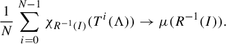 $$ \begin{align*}\frac{1}{N}\sum_{i=0} ^{N-1}\chi_{ R^{-1}(I)}(T^i(\Lambda))\to \mu(R^{-1}(I)).\end{align*} $$
Since the cumulative distribution function is given by the total area bounded by the return time hyperbolas, it is piecewise real analytic. In particular, it is continuous and differentiable. The probability density associated with the slope gap is simply the derivative of the cumulative distribution function. For example, for
 $m_\Omega $
-generic points, we have the probability density is given by
$m_\Omega $
-generic points, we have the probability density is given by
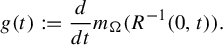 $$ \begin{align*}g(t) := \frac{d}{dt}m_\Omega(R^{-1}(0,t)).\end{align*} $$
Hence, the proportion of gaps in an interval I of an
 $m_\Omega $
-generic affine lattice
$m_\Omega $
-generic affine lattice
 $\Lambda \in \Omega $
is given by
$\Lambda \in \Omega $
is given by
 $$ \begin{align*}\lim_{N\to\infty}\frac{1}{N}|\mathcal G^N _V(\Lambda)\cap I|=\lim_{N\to\infty}\frac{1}{N}\sum_{i=0} ^{N-1}\chi_{ R^{-1}(I)}(T^i(\Lambda))= m_\Omega(R^{-1}(I))=\int_I g(t) \,dt.\end{align*} $$
Similarly, for
 $m_q$
-generic points, we have the probability density is given by
$m_q$
-generic points, we have the probability density is given by
 $$ \begin{align*}g_q(t) := \frac{d}{dt}m_q(R^{-1}(0,t))\end{align*} $$
and the proportion of gaps given by
 $$ \begin{align*}\lim_{N\to\infty}\frac{1}{N}|\mathcal G^N _V(\Lambda)\cap I|=\int_I g_q(t) \,dt.\\[-40pt]\end{align*} $$
Proof Proof of Theorem 2.1
A similar argument works to prove that the slope gap limit (5) for doubled slit tori exists for any
 $m_{\mathcal W}$
-generic point of
$m_{\mathcal W}$
-generic point of
 $\mathcal W$
. Indeed,
$\mathcal W$
. Indeed,
 $$ \begin{align*}\lim_{N\to\infty}\frac{1}{N}|\mathcal G^N _V(\Lambda_\omega)\cap I|=\lim_{N\to\infty}\frac{1}{N}\sum_{i=0} ^{N-1}\chi_{\mathcal R^{-1}(I)}(\mathcal T^{{\kern2pt}i}(\Lambda_\omega)) =m_{{\mathcal{W}}}(\mathcal R^{-1}(I)).\end{align*} $$
This proves Theorem 1.1. The probability density associated with the slope gap is simply the derivative of the cumulative distribution function. We denote this density by f. That is,
 $$ \begin{align*}f(t) := \frac{d}{dt}m_{\mathcal{W}}(\mathcal R^{-1}(0,t)),\end{align*} $$
where
 $\mathcal R$
is the first return map to
$\mathcal R$
is the first return map to
 ${\mathcal {W}}.$
Hence, the proportion of gaps of saddle connections in an interval I of an
${\mathcal {W}}.$
Hence, the proportion of gaps of saddle connections in an interval I of an
 $m_{\mathcal {W}}$
-generic translation surface
$m_{\mathcal {W}}$
-generic translation surface
 $\omega \in {\mathcal {W}}$
is given by
$\omega \in {\mathcal {W}}$
is given by
 $$ \begin{align*}\lim_{N\to\infty}\frac{1}{N}|\mathcal G^N _V(\Lambda_\omega)\cap I|=\int_I f(t) \,dt.\\[-40pt]\end{align*} $$
We state more precisely the conclusions of the above theorems now as well. Recall that
 $F\sim G$
means that for large enough t, the ratio is a positive constant and
$F\sim G$
means that for large enough t, the ratio is a positive constant and
 $F\ll G$
means there is a positive constant c so that for large enough t,
$F\ll G$
means there is a positive constant c so that for large enough t,
 $|F(t)|\le c|G(t)|$
.
$|F(t)|\le c|G(t)|$
.
Theorem 4.4.
-
(1) For any affine lattice in
$ \Omega $
that is generic for
$m_{\Omega }$
, we have that the proportion of gaps larger than t, satisfies
$$ \begin{align*}\int_t ^\infty g(t)\,dt\end{align*} $$
Here
$$ \begin{align*}t^{-2}\ll\int_t ^\infty g(t)\,dt\ll t^{-1}.\end{align*} $$
$g(t)$
is the density function for affine lattices from the proof of Theorem 2.2.
-
(2) There is support at zero for any affine lattice in
$ \Omega $
that is generic for
$m_{\Omega }$
. That is, for any
$\varepsilon>0$
,
$$ \begin{align*}\int_0 ^\varepsilon g(t)\,dt>0.\end{align*} $$
-
(3) For any doubled slit torus in
${\mathcal {W}}$
that is generic with respect to
$m_{\mathcal {W}}$
, we have that the proportion of gaps of saddle connections larger than t decays quadratically. More precisely, Here,
$$ \begin{align*}\int_t ^\infty f(t)\,dt\sim t^{-2}.\end{align*} $$
$f(t)$
is the density function for doubled slit tori from the proof of Theorem 1.1.
-
(4) There is support at zero for any doubled slit torus in
$ {\mathcal {W}}$
that is generic with respect to
$m_{\mathcal {W}}$
. That is, for any
$\varepsilon>0$
,
$$ \begin{align*}\int_0 ^\varepsilon f(t)\,dt>0.\end{align*} $$


Remark 4.5. While the statements in part (1) of Theorem 4.4 are for gaps of affine lattices that are already in the transversal
 $\Omega $
and generic for
$\Omega $
and generic for
 $m_\Omega $
, we can obtain information about the gaps of an affine lattice
$m_\Omega $
, we can obtain information about the gaps of an affine lattice
 $\Lambda $
that is generic for
$\Lambda $
that is generic for
 $m_{AX_2}$
. Let
$m_{AX_2}$
. Let
 $\Lambda '\in \Omega $
be such that
$\Lambda '\in \Omega $
be such that
 $h_u\Lambda = \Lambda '$
and u is the smallest time for which this occurs. Then,
$h_u\Lambda = \Lambda '$
and u is the smallest time for which this occurs. Then,
 $$ \begin{align*}\lim_{R\to\infty}\frac{| \mathcal G^R _V(\Lambda )\cap (t,\infty)|}{N(R)}= \lim_{R\to\infty}\frac{| \mathcal G^R _V(\Lambda' )\cap (t,\infty)|}{N(R)}=\int_t ^\infty g(t)\,dt.\end{align*} $$
Similar arguments can be used for the rest of Theorem 4.4 to turn statements about the transversal to statements about the ambient space.
4.4 d-Symmetric torus covers
We can apply our results of doubled slit tori to a more general class of translation surfaces. Let
 $d>1$
and consider d-copies of a torus X that we label
$d>1$
and consider d-copies of a torus X that we label
 $X_1,\ldots ,X_d$
. Now glue the copies along a slit and identify opposite sides of the slits according to the permutation
$X_1,\ldots ,X_d$
. Now glue the copies along a slit and identify opposite sides of the slits according to the permutation
 $(1,2,\ldots , d)$
. Following [Reference Schmoll26], we call a surface constructed in this way a d-symmetric torus cover. Notice that a doubled slit torus simply corresponds to this construction with
$(1,2,\ldots , d)$
. Following [Reference Schmoll26], we call a surface constructed in this way a d-symmetric torus cover. Notice that a doubled slit torus simply corresponds to this construction with
 $d=2$
.
$d=2$
.
Any d-symmetric torus cover has two cone points of angle
 $2d\pi $
and has genus d. Let
$2d\pi $
and has genus d. Let
 ${\mathcal {E}}^d$
denote the class d-symmetric torus covers. We have
${\mathcal {E}}^d$
denote the class d-symmetric torus covers. We have
 ${\mathcal {E}}^d\subset \mathcal H(d-1,d-1)$
. See Figure 4 for an example of a d-symmetric torus cover.
${\mathcal {E}}^d\subset \mathcal H(d-1,d-1)$
. See Figure 4 for an example of a d-symmetric torus cover.
An example of a d-symmetric torus cover.
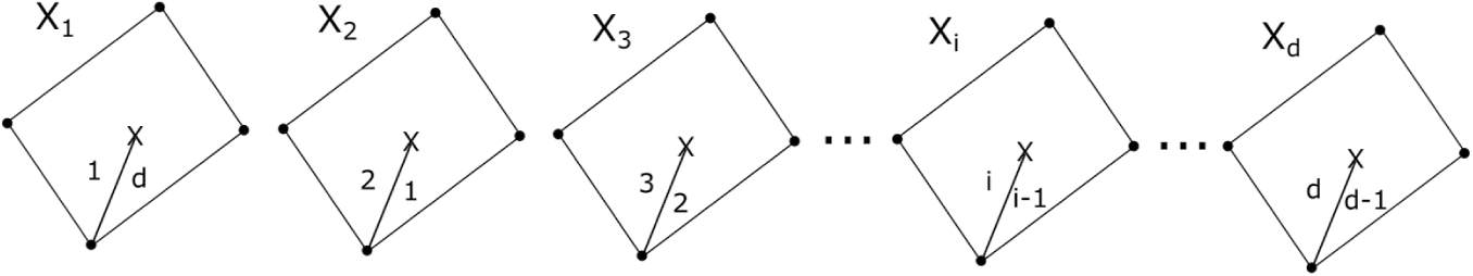
We remark that we can do a similar construction with any cycle
 $\sigma \in S^d$
(cycle so that the resulting surface is connected). By relabeling the d-copies, there is no loss in generality in assuming
$\sigma \in S^d$
(cycle so that the resulting surface is connected). By relabeling the d-copies, there is no loss in generality in assuming
 $(1,2,\ldots , d)$
.
$(1,2,\ldots , d)$
.
The results for doubled slit tori allow us to compute the gap distribution of a typical element in
 ${\mathcal {E}}^d$
. In particular, this yields an explicit gap distribution for a translation surface in any genus
${\mathcal {E}}^d$
. In particular, this yields an explicit gap distribution for a translation surface in any genus
 $d>1$
.
$d>1$
.
Corollary 4.6. For
 $d>1$
, the gap distribution of a d-symmetric torus cover can be computed using the density function for doubled slit tori. That is,
$d>1$
, the gap distribution of a d-symmetric torus cover can be computed using the density function for doubled slit tori. That is,
 $$ \begin{align*}\lim_{R\to\infty}\frac{| \mathcal G^R (\Lambda_\omega) \cap I|}{N(\omega, R)}=\int_I f(x)\,dx\end{align*} $$
for almost every
 $\omega \in {\mathcal {E}}^d$
with respect to an
$\omega \in {\mathcal {E}}^d$
with respect to an
 ${\textrm {SL}}_2({\mathbb {R}})$
-invariant probability measure on
${\textrm {SL}}_2({\mathbb {R}})$
-invariant probability measure on
 ${\mathcal {E}}^d$
that is in the same measure class as the Lebesgue measure. Here,
${\mathcal {E}}^d$
that is in the same measure class as the Lebesgue measure. Here,
 $f(t)$
is the density function for doubled slit tori from the proof of Theorem 1.1.
$f(t)$
is the density function for doubled slit tori from the proof of Theorem 1.1.
Proof Consider a typical element
 $\omega _1\in {\mathcal {E}}^d$
. We obtain a twice-marked torus
$\omega _1\in {\mathcal {E}}^d$
. We obtain a twice-marked torus
 $(g,v)\in \mathcal H(0,0)$
by projecting to a single copy and forgetting the slit. Use this twice-marked torus to construct a doubled slit torus
$(g,v)\in \mathcal H(0,0)$
by projecting to a single copy and forgetting the slit. Use this twice-marked torus to construct a doubled slit torus
 $\omega _2$
. Each has the same set of saddle connections (
$\omega _2$
. Each has the same set of saddle connections (
 $\Lambda _{\omega _1} = \Lambda _{\omega _2})$
so that their respective gap distributions are the same as well.
$\Lambda _{\omega _1} = \Lambda _{\omega _2})$
so that their respective gap distributions are the same as well.
Acknowledgments
This research was supported by the National Science Foundation Graduate Research Fellowship under Grant No. 1122374. This paper is part of my thesis and I would like to give many thanks to my advisor Jayadev Athreya for his continuous encouragement and endless patience. I thank Dami Lee and Sunrose Shrestha for useful comments on the paper and Aaron Calderon, Martin Schmoll, and Jane Wang for helpful discussions. I also thank Jane Wang for pointing out a mistake in my measure classification theorem. I am indebted to the referee for a careful reading of the manuscript and several comments and suggestions that improved my paper.
A Appendix. Measure computations and estimates
In the appendix we compute an explicit limiting gap distribution for slopes of saddle connections on a doubled slit torus. We also prove estimates on the decay of gaps for affine lattices.
A.1 Haar-measure computations and estimates for
${\mathcal {W}}$

In this section, we explicitly calculate the gap distribution function given by
 $$ \begin{align*}m_{{\mathcal{W}}}(\omega\in {\mathcal{W}}| \mathcal R(\omega)>t),\end{align*} $$
where
 $t>0$
. As a corollary, we compute the decay rate of the tail and show there is support at zero.
$t>0$
. As a corollary, we compute the decay rate of the tail and show there is support at zero.
We compute the distribution by considering the partition on
 ${\mathcal {W}}$
given by surfaces with projection of a short affine lattice
${\mathcal {W}}$
given by surfaces with projection of a short affine lattice
 ${\mathcal {W}}_{\mathrm{sa}}$
and surfaces with projection of a short lattice
${\mathcal {W}}_{\mathrm{sa}}$
and surfaces with projection of a short lattice
 ${\mathcal {W}}_{\mathrm{sl}}$
. On either part of the partition, we will have the return time map
${\mathcal {W}}_{\mathrm{sl}}$
. On either part of the partition, we will have the return time map
 $\mathcal R$
explicitly. The basic idea of proof will be to use the condition of there being a gap larger than t (i.e that the return time
$\mathcal R$
explicitly. The basic idea of proof will be to use the condition of there being a gap larger than t (i.e that the return time
 $\mathcal R$
is larger than t) and see what conditions are imposed on the coordinates where the return time is defined. This will yield explicit integrals whence we can compute the integrals and make arguments with a Taylor series to show their decay.
$\mathcal R$
is larger than t) and see what conditions are imposed on the coordinates where the return time is defined. This will yield explicit integrals whence we can compute the integrals and make arguments with a Taylor series to show their decay.
A.1.1 Haar-measure computations and estimates for
${\mathcal {W}}_{\mathrm{sa}}$

We compute the contribution on the doubled slit tori coming from a short affine piece. That is,
 $$ \begin{align*}m_{\mathcal W}(\{\omega\in {\mathcal{W}}_{\mathrm{sa}}| \mathcal R(\omega)>t\}) .\end{align*} $$
The return time map
 $\mathcal R$
is a piecewise map on three pieces depending on
$\mathcal R$
is a piecewise map on three pieces depending on
 $\Pi (\omega )$
. In each piece, we know explicitly the return map and so we can compute the contribution.
$\Pi (\omega )$
. In each piece, we know explicitly the return map and so we can compute the contribution.
Contribution when
 $\Pi (\omega )\in \Omega _1.$
Suppose
$\Pi (\omega )\in \Omega _1.$
Suppose
 $\Pi (\omega )\in \Omega _1.$
Notice that
$\Pi (\omega )\in \Omega _1.$
Notice that
 $\Omega _1$
can be written as
$\Omega _1$
can be written as
 $$ \begin{align*}\Omega_1 = \bigg\{(a,b,s,{\alpha})\in \Omega: b\in(0,1], {\alpha}\in(1-b,1], a\in(1-b,{\alpha}], s\in\bigg[0,\frac{{\alpha}-a}{ab{\alpha}}\bigg)\bigg\}.\end{align*} $$
We have,
 $$ \begin{align*}m_{{\mathcal{W}}}(\{\omega\in {\mathcal{W}}_{\mathrm{sa}}| \mathcal R(\omega)>t, \Pi(\omega)\in \Omega_1\}) = 4 m_{\Omega}(\{(a,b,s,{\alpha})\in\Omega_1:R(a,b,s,{\alpha})>t\}) .\end{align*} $$
Thus, we now compute
 $m_{\Omega }(\Omega _1\cap \{R>t\}) .$
The condition on the return time says
 $$ \begin{align*}t<R(a,b,s,\alpha) = \frac{sa}{{\alpha}-a}\iff \frac{t({\alpha}-a)}{a}<s.\end{align*} $$
Notice that this is a valid lower bound for s since s is non-negative. On
 $\Omega _1$
, s has an upper bound of
$\Omega _1$
, s has an upper bound of
 $({{\alpha }-a})/{ab{\alpha }}$
so in order for the return map R to be larger than t, we must also satisfy the cross-term condition
$({{\alpha }-a})/{ab{\alpha }}$
so in order for the return map R to be larger than t, we must also satisfy the cross-term condition
 $ {t({\alpha }-a)}/{a}<s< ({{\alpha }-a})/{ab{\alpha }}\iff t<{1}/{b{\alpha }}$
. We rewrite this as
$ {t({\alpha }-a)}/{a}<s< ({{\alpha }-a})/{ab{\alpha }}\iff t<{1}/{b{\alpha }}$
. We rewrite this as
 ${\alpha }<{1}/{bt}$
. Hence, all we need to understand is how the hyperbola
${\alpha }<{1}/{bt}$
. Hence, all we need to understand is how the hyperbola
 ${\alpha }=1/bt$
intersects the
${\alpha }=1/bt$
intersects the
 $(b,{\alpha })$
-triangle
$(b,{\alpha })$
-triangle
 $\{(b,{\alpha }): b\in (0,1], {\alpha }\in (1-b,1]\}$
. See Figure A1 for an illustration for the
$\{(b,{\alpha }): b\in (0,1], {\alpha }\in (1-b,1]\}$
. See Figure A1 for an illustration for the
 $(b,a)$
slice of the contribution of
$(b,a)$
slice of the contribution of
 $\Omega _1$
when
$\Omega _1$
when
 $t>4$
.
$t>4$
.
The contribution on
 $\Omega _1$
when
$\Omega _1$
when
 $t>4$
.
$t>4$
.
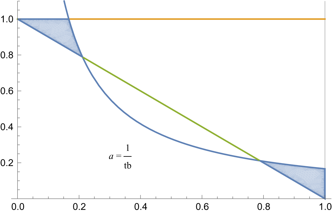
If
 $t\in (0,1)$
, then everything lies below the hyperbola
$t\in (0,1)$
, then everything lies below the hyperbola
 ${\alpha }={1}/{bt}$
and our contribution is given by
${\alpha }={1}/{bt}$
and our contribution is given by
 $$ \begin{align*}m_{\Omega}(\{R>t\}\cap \Omega_1)=\int _{b=0} ^{1} \int_{{\alpha}=1-b} ^{1} \int_{a=1-b} ^ {\alpha} \int _{s={t({\alpha}-a)}/{a}} ^{({{\alpha}-a})/{ab{\alpha}}} 1\,ds\,da\,d{\alpha}\,db.\end{align*} $$
If
 $t\in [1,4)$
, then
$t\in [1,4)$
, then
 $$ \begin{align*} m_{\Omega}(\{R>t\}\cap \Omega_1)&= \int _{b=0} ^{1/t} \int_{{\alpha}=1-b} ^{1} \int_{a=1-b} ^ {\alpha} \int _{s={t({\alpha}-a)}/{a}} ^{({{\alpha}-a})/{ab{\alpha}}} 1\,ds\,da\,d{\alpha}\,db\\ &\quad+ \int _{b=1/t} ^{1} \int_{{\alpha}=1-b} ^{1/bt} \int_{a=1-b} ^ {\alpha} \int _{s={t({\alpha}-a)}/{a}} ^{({{\alpha}-a})/{ab{\alpha}}} 1\,ds\,da\,d{\alpha}\,db. \end{align*} $$
If
 $t\in [4,\infty )$
, then
$t\in [4,\infty )$
, then
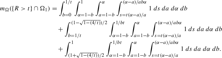 $$ \begin{align*} m_{\Omega}(\{R>t\}\cap \Omega_1)& =\int_{b=0}^{1/t}\int_{{\alpha}=1-b}^{1}\int_{a=1-b}^{{\alpha}}\int _{s={t({\alpha}-a)}/{a}} ^{({{\alpha}-a})/{ab{\alpha}}}1\,ds\,da\,d{\alpha}\,db \\ &\quad+ \int _{b=1/t} ^{({1-\sqrt{1-(4/t)}})/{2}} \int_{{\alpha}=1-b} ^{1/bt} \int_{a=1-b} ^ {\alpha} \int _{s={t({\alpha}-a)}/{a}} ^{({{\alpha}-a})/{ab{\alpha}}} 1\,ds\,da\,d{\alpha}\,db\\ &\quad+ \int _{({1+\sqrt{1-(4/t)}})/{2}}^1 \int_{{\alpha}=1-b} ^{1/bt} \int_{a=1-b} ^ {\alpha} \int _{s={t({\alpha}-a)}/{a}} ^{({{\alpha}-a})/{ab{\alpha}}} 1\,ds\,da\,d{\alpha}\,db. \end{align*} $$
By evaluating each integral and then approximating the result by its Taylor series, we can understand how it decays. As an example, we do this for the first integral.
 $$ \begin{align*} &\int_{b=0}^{1/t}\int_{{\alpha}=1-b}^{1}\int_{a=1-b}^{{\alpha}}\int _{s={t({\alpha}-a)}/{a}} ^{({{\alpha}-a})/{ab{\alpha}}}1\,ds\,da\,d{\alpha} \,db\\ &\quad= \int_{b=0}^{1/t}\frac{ b(b (2 + b) t-8) + 2 ( b (2 + t)-4) \log(1 - b)}{4b}\,db\\ &\quad\approx \int_{b=0}^{1/t}\frac{ b( b (2 + b) t-8) + 2 ( b (2 + t)-4)(-b -({ b^2}/{2}) -({ b^3}/{3}))}{4b}\,db \\ &\quad=- \frac{1}{6} \int_{b=0}^{1/t}b^2 ( b (2 + t)-1)\,db = -\frac{1}{12 t^4} + \frac{1}{72 t^3}. \end{align*} $$
Hence, on this piece, we have a cubic decay. Doing this for the rest of the integrals, we have
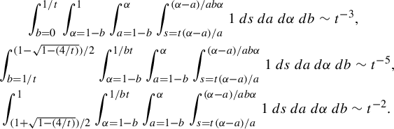 $$ \begin{align*} \int_{b=0}^{1/t}\int_{{\alpha}=1-b}^{1}\int_{a=1-b}^{{\alpha}}\int _{s={t({\alpha}-a)}/{a}} ^{({{\alpha}-a})/{ab{\alpha}}}1\,ds\,da\,d{\alpha} \,db\sim t^{-3},\qquad\quad \\ \int _{b=1/t} ^{({1-\sqrt{1-(4/t)}})/{2}} \int_{{\alpha}=1-b} ^{1/bt} \int_{a=1-b} ^ {\alpha} \int _{s={t({\alpha}-a)}/{a}} ^{({{\alpha}-a})/{ab{\alpha}}} 1\,ds\,da\,d{\alpha} \,db\sim t^{-5}, \ \, \\ \int _{({1+\sqrt{1-(4/t)}})/{2}}^1 \int_{{\alpha}=1-b} ^{1/bt} \int_{a=1-b} ^ {\alpha} \int _{s={t({\alpha}-a)}/{a}} ^{({{\alpha}-a})/{ab{\alpha}}} 1\,ds\,da\,d{\alpha} \,db\sim t^{-2}. \ \ \, \end{align*} $$
Hence, the decay rate on the tail of
 $\Omega _1$
is quadratic. By multiplying each integral above by 4, we have that contribution of
$\Omega _1$
is quadratic. By multiplying each integral above by 4, we have that contribution of
 $$ \begin{align*}m_{\mathcal W}(\{\omega\in {\mathcal{W}}_{\mathrm{sa}}| \mathcal R(\omega)>t,\Pi(\omega)\in\Omega_1\})\end{align*} $$
and also the decay rate
 $$ \begin{align*}m_{\mathcal W}(\{\omega\in {\mathcal{W}}_{\mathrm{sa}}| \mathcal R(\omega)>t,\Pi(\omega)\in\Omega_1\}) \sim t^{-2}.\end{align*} $$
Contribution when
 $\Pi (\omega )\in \Omega _3.$
Suppose
$\Pi (\omega )\in \Omega _3.$
Suppose
 $\Pi (\omega )\in \Omega _3.$
Notice that
$\Pi (\omega )\in \Omega _3.$
Notice that
 $\Omega _3$
can be written as
$\Omega _3$
can be written as
 $$ \begin{align*}\Omega_3 = \bigg\{(a,b,s,{\alpha})\in \Omega: b\in(0,1], {\alpha}\in(0,1-b], a\in(1-b,1], s\in\bigg[0,\frac{1}{ab}\bigg)\bigg\}.\end{align*} $$
We have
 $$ \begin{align*}m_{{\mathcal{W}}}(\{\omega\in {\mathcal{W}}_{\mathrm{sa}}| \mathcal R(\omega)>t, \Pi(\omega)\in \Omega_3\}) = 4 m_{\Omega}(\{(a,b,s,{\alpha})\in\Omega_3:R(a,b,s,{\alpha})>t\}) .\end{align*} $$
Thus, we now compute
 $m_{\Omega }(\Omega _3\cap \{R>t\}) .$
On
 $\Omega _3$
, we have
$\Omega _3$
, we have
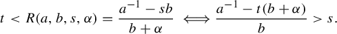 $$ \begin{align*}t<R(a,b,s,\alpha) =\frac{a^{-1}-sb}{b+{\alpha}}\iff \frac{a^{-1}-t(b+{\alpha})}{b}>s.\end{align*} $$
Notice that the left-hand side is always bounded above by
 $(ab)^{-1}.$
In order for there to be any valid values, we need the left-hand side to be positive, which is equivalent to
$(ab)^{-1}.$
In order for there to be any valid values, we need the left-hand side to be positive, which is equivalent to
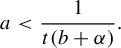 $$ \begin{align*}a<\frac{1}{t(b+{\alpha})}.\end{align*} $$
Hence, we seek the minimum between
 ${1}/{t(b+{\alpha })}$
and a.
${1}/{t(b+{\alpha })}$
and a.
Case I:
 $a<\min \{{1}/{t(b+{\alpha })},1\} =1$
. This happens when
$a<\min \{{1}/{t(b+{\alpha })},1\} =1$
. This happens when
 $$ \begin{align*}\frac{1}{t(b+{\alpha})}>1 \iff {\alpha}<\frac{1}{t}-b.\end{align*} $$
Notice now that
 ${\alpha }<1-b$
on
${\alpha }<1-b$
on
 $\Omega _3$
and that
$\Omega _3$
and that
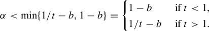 $$ \begin{align*}{\alpha}<\min\{1/t-b,1-b\}=\begin{cases} 1-b &\text{ if } t<1,\\ 1/t-b &\text{ if } t>1. \end{cases}\end{align*} $$
Hence, if
 $t<1$
, the integral is
$t<1$
, the integral is
 $$ \begin{align*}\int_{b=0} ^{1} \int_{{\alpha}=0} ^{1-b}\int_{a=1-b} ^1 \int _{s=0} ^{({a^{-1}-t(b+{\alpha})})/{b}}1\,ds\,da\,d{\alpha} \,db = \frac{\pi^2}{6} -1 - \frac{ t}{3}.\end{align*} $$
On the other hand, if
 $t>1$
, then
$t>1$
, then
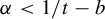 ${\alpha }<1/t-b$
and since
${\alpha }<1/t-b$
and since
 ${\alpha }>0$
, we must have
${\alpha }>0$
, we must have
 $1/t>b$
. Thus, for large t (larger than 1), the integral is
$1/t>b$
. Thus, for large t (larger than 1), the integral is
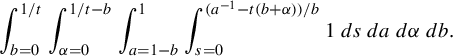 $$ \begin{align*}\int_{b=0} ^{1/t} \int_{{\alpha}=0} ^{1/t-b}\int_{a=1-b} ^1 \int _{s=0} ^{({a^{-1}-t(b+{\alpha})})/{b}}1\,ds\,da\,d{\alpha} \,db.\end{align*} $$
A Taylor series argument shows that this decays quadratically.
Case II:
 $a<\min \{{1}/{t(b+{\alpha })},1\} = {1}/{t(b+{\alpha })}$
. This happens when
$a<\min \{{1}/{t(b+{\alpha })},1\} = {1}/{t(b+{\alpha })}$
. This happens when
 $$ \begin{align*}\frac{1}{t(b+{\alpha})}<1 \iff {\alpha}>\frac{1}{t}-b.\end{align*} $$
Since
 $1-b<{\alpha }$
, then combining the inequalities, we obtain
$1-b<{\alpha }$
, then combining the inequalities, we obtain
 $$ \begin{align*}{\alpha}<\frac{b^2-b+1/t}{1-b}.\end{align*} $$
By understanding how these functions intersect the
 $(b,{\alpha })$
-plane
$(b,{\alpha })$
-plane
 $$ \begin{align*}\{(b,{\alpha})\mid 0<b\le1\text{ and }0<{\alpha}<1-b\},\end{align*} $$
then we can understand how this function grows in t.
We obtain the following. If
 $t\in (0,1)$
, there is no contribution.
$t\in (0,1)$
, there is no contribution.
If
 $t\in [1,2)$
, the contribution is
$t\in [1,2)$
, the contribution is
 $$ \begin{align*} &m_{\Omega}(\{R>t\}\cap \Omega_3)\\ &\quad=\int_{b=0} ^{1-1/t} \int_{{\alpha}=1/t - b} ^{({b^2-b+1/t})/({1-b})} \int_{a=1-b} ^{1/(t(b+{\alpha}))} \int _{s=0} ^{({a^{-1}-t(b+{\alpha})})/{b}} 1\,ds\,da\,d{\alpha}\,db\\ &\qquad+\int_{b=1-1/t} ^{1/t} \int_{{\alpha}=1/t - b} ^{1-b} \int_{a=1-b} ^{1/(t(b+{\alpha}))} \int _{s=0} ^{({a^{-1}-t(b+{\alpha})})/{b}} 1\,ds\,da\,d{\alpha}\,db\\ &\qquad+\int_{b=1/t} ^{1} \int_{{\alpha}=0} ^{1-b} \int_{a=1-b} ^{1/(t(b+{\alpha}))} \int _{s=0} ^{({a^{-1}-t(b+{\alpha})})/{b}} 1\,ds\,da\,d{\alpha}\,db. \end{align*} $$
If
 $t\in [2,4)$
, the contribution is
$t\in [2,4)$
, the contribution is
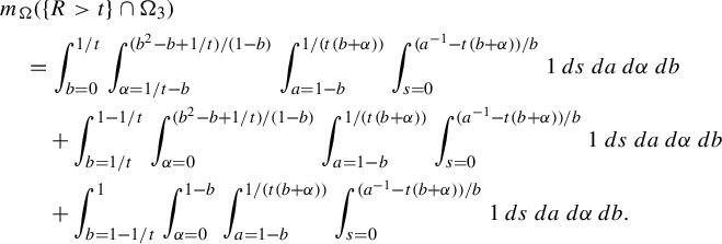 $$ \begin{align*} &m_{\Omega}(\{R>t\}\cap \Omega_3)\\ &\quad=\int_{b=0} ^{1/t} \int_{{\alpha}=1/t - b} ^{({b^2-b+1/t})/({1-b})} \int_{a=1-b} ^{1/(t(b+{\alpha}))} \int _{s=0} ^{({a^{-1}-t(b+{\alpha})})/{b}} 1\,ds\,da\,d{\alpha}\,db\\ &\qquad+\int_{b=1/t} ^{1-1/t} \int_{{\alpha}=0} ^{({b^2-b+1/t})/({1-b})} \int_{a=1-b} ^{1/(t(b+{\alpha}))} \int _{s=0} ^{({a^{-1}-t(b+{\alpha})})/{b}} 1\,ds\,da\,d{\alpha}\,db\\ &\qquad+\int_{b=1-1/t} ^{1} \int_{{\alpha}=0} ^{1-b} \int_{a=1-b} ^{1/(t(b+{\alpha}))} \int _{s=0} ^{({a^{-1}-t(b+{\alpha})})/{b}} 1\,ds\,da\,d{\alpha}\,db. \end{align*} $$
If
 $t>4$
, the tail on this piece of
$t>4$
, the tail on this piece of
 $\Omega _3$
is given by
$\Omega _3$
is given by
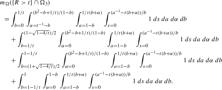 $$ \begin{align*} m_{\Omega}&(\{R>t\}\cap \Omega_3)\\=&\int_{b=0} ^{1/t}\int_{{\alpha}=t^{-1}-b} ^{({b^2-b+1/t})/({1-b})}\int_{a=1-b} ^{1/t(b+{\alpha})}\int_{s=0} ^{({a^{-1}-t(b+{\alpha})})/{b}}1\,ds\,da\,d{\alpha} \,db \\ &+ \int_{b=1/t} ^{({1-\sqrt{1-4/t}})/{2}}\int_{{\alpha}=0} ^{({b^2-b+1/t})/({1-b})}\int_{a=1-b} ^{1/t(b+{\alpha})}\int_{s=0} ^{({a^{-1}-t(b+{\alpha})})/{b}}1\,ds\,da\,d{\alpha}\, db\\ &+\int_{b=({1+\sqrt{1-4/t}})/{2}} ^{1-1/t} \int_{{\alpha}=0} ^{({b^2-b+1/t})/({1-b})}\int_{a=1-b} ^{1/t(b+{\alpha})}\int_{s=0} ^{({a^{-1}-t(b+{\alpha})})/{b}}1\,ds\,da\,d{\alpha} \,db\\ &+\int_{b=1-1/t} ^{1} \int_{{\alpha}=0} ^{1-b} \int_{a=1-b} ^{1/t(b+{\alpha})}\int_{s=0} ^{({a^{-1}-t(b+{\alpha})})/{b}}1\,ds\,da\,d{\alpha} \,db. \end{align*} $$
By evaluating each integral and then approximating by its Taylor series, we see that
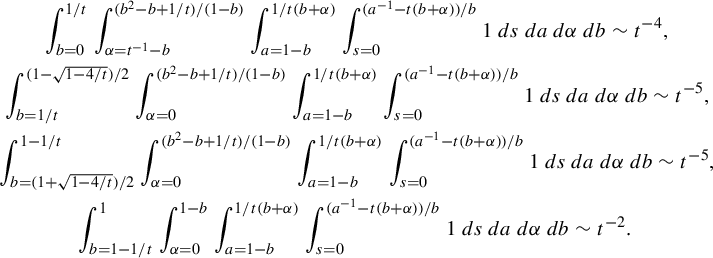 $$ \begin{align*} \int_{b=0} ^{1/t}\int_{{\alpha}=t^{-1}-b} ^{({b^2-b+1/t})/({1-b})}\int_{a=1-b} ^{1/t(b+{\alpha})}\int_{s=0} ^{({a^{-1}-t(b+{\alpha})})/{b}}1\,ds\,da\,d{\alpha} \,db \sim t^{-4}, \qquad \ \\ \int_{b=1/t} ^{({1-\sqrt{1-4/t}})/{2}}\int_{{\alpha}=0} ^{({b^2-b+1/t})/({1-b})}\int_{a=1-b} ^{1/t(b+{\alpha})}\int_{s=0} ^{({a^{-1}-t(b+{\alpha})})/{b}}1\,ds\,da\,d{\alpha}\, db\sim t^{-5},\ \\ \int_{b=({1+\sqrt{1-4/t}})/{2}} ^{1-1/t} \int_{{\alpha}=0} ^{({b^2-b+1/t})/({1-b})}\int_{a=1-b} ^{1/t(b+{\alpha})}\int_{s=0} ^{({a^{-1}-t(b+{\alpha})})/{b}}1\,ds\,da\,d{\alpha} \,db\sim t^{-5},\\ \int_{b=1-1/t} ^{1} \int_{{\alpha}=0} ^{1-b} \int_{a=1-b} ^{1/t(b+{\alpha})}\int_{s=0} ^{({a^{-1}-t(b+{\alpha})})/{b}}1\,ds\,da\,d{\alpha} \,db\sim t^{-2}.\qquad\qquad \end{align*} $$
By adding the contributions from both cases, we conclude that
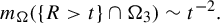 $$ \begin{align*}m_{\Omega}(\{R>t\}\cap \Omega_3)\sim t^{-2}.\end{align*} $$
By multiplying each integral above by 4, we have that contribution of
 $$ \begin{align*}m_{\mathcal W}(\{\omega\in {\mathcal{W}}_{\mathrm{sa}}| \mathcal R(\omega)>t,\Pi(\omega)\in\Omega_3\})\end{align*} $$
and also the decay rate
 $$ \begin{align*}m_{\mathcal W}(\{\omega\in {\mathcal{W}}_{\mathrm{sa}}| \mathcal R(\omega)>t,\Pi(\omega)\in\Omega_3\}) \sim t^{-2}.\end{align*} $$
Contribution when
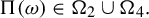 $\Pi (\omega )\in \Omega _2 \cup \Omega _4.$
Suppose
$\Pi (\omega )\in \Omega _2 \cup \Omega _4.$
Suppose
 $\Pi (\omega )\in \Omega _2$
. Notice that
$\Pi (\omega )\in \Omega _2$
. Notice that
 $\Omega _2$
can be written as
$\Omega _2$
can be written as
 $$ \begin{align*}\Omega_2=\bigg\{b\in(0,1],{\alpha}\in(1-b,1],a\in(1-b,{\alpha}),s\in\bigg[(ab)^{-1}\bigg(\frac{{\alpha}-a}{{\alpha}}\bigg),(ab)^{-1}\bigg)\bigg\}.\end{align*} $$
We have
 $$ \begin{align*}m_{{\mathcal{W}}}(\{\omega\in {\mathcal{W}}_{\mathrm{sa}}| \mathcal R(\omega)>t, \Pi(\omega)\in \Omega_2\}) = 4 m_{\Omega}(\{(a,b,s,{\alpha})\in\Omega_2: (ab)^{-1}-s>t\}) .\end{align*} $$
Unpacking a little, we see
 $$ \begin{align*}(ab)^{-1}-s>t \iff (ab)^{-1}-t>s\end{align*} $$
and this is always the minimum upper bound for s in
 $\Omega _2$
since
$\Omega _2$
since
 $t>0$
. On the other hand, to satisfy the cross-term condition, we need
$t>0$
. On the other hand, to satisfy the cross-term condition, we need
 $$ \begin{align*}(ab)^{-1}\bigg(\frac{{\alpha}-a}{{\alpha}}\bigg)<(ab)^{-1}-t \iff{\alpha}<1/bt.\end{align*} $$
Hence, we want to understand how the hyperbola
 ${\alpha }=1/bt$
intersects the triangle
${\alpha }=1/bt$
intersects the triangle
 $$ \begin{align*}\{(b,{\alpha})\mid b\in(0,1],{\alpha}\in(1-b,1]\}.\end{align*} $$
If
 $t\in [0,1)$
, then everything lies below the hyperbola
$t\in [0,1)$
, then everything lies below the hyperbola
 ${\alpha }={1}/{bt}$
and the contribution is
${\alpha }={1}/{bt}$
and the contribution is
 $$ \begin{align*}m_{\Omega}(\{\mathcal R>t\}\cap\Omega_2)=\int _{b=0} ^{1} \int_{{\alpha}=1-b} ^{1} \int_{a=1-b} ^ {\alpha} \int _{s=(ab)^{-1}(({{\alpha}-a})/{{\alpha}})} ^{(ab)^{-1}-t} 1\,ds\,da\,d{\alpha}\,db.\end{align*} $$
If
 $t\in [1,4)$
, then the hyperbola
$t\in [1,4)$
, then the hyperbola
 ${\alpha }={1}/{bt}$
intersects once at
${\alpha }={1}/{bt}$
intersects once at
 $b=1/t$
and the contribution is
$b=1/t$
and the contribution is
 $$ \begin{align*} m_{\Omega}(\{\mathcal R>t\}\cap\Omega_2)&= \int _{b=0} ^{1/t} \int_{{\alpha}=1-b} ^{1} \int_{a=1-b} ^ {\alpha} \int _{s=(ab)^{-1}(({{\alpha}-a})/{{\alpha}})} ^{(ab)^{-1}-t} 1\,ds\,da\,d{\alpha}\,db \\ &\quad+ \int _{b=1/t} ^{1} \int_{{\alpha}=1-b} ^{1/bt} \int_{a=1-b} ^ {\alpha} \int _{s=(ab)^{-1}(({{\alpha}-a})/{{\alpha}})} ^{(ab)^{-1}-t} 1\,ds\,da\,d{\alpha} \,db. \end{align*} $$
If
 $t\in [4,\infty )$
, then the hyperbola
$t\in [4,\infty )$
, then the hyperbola
 ${\alpha }={1}/{bt}$
intersects twice and the contribution is
${\alpha }={1}/{bt}$
intersects twice and the contribution is
 $$ \begin{align*} m_{\Omega}&(\{\mathcal R>t\}\cap\Omega_2)\\ &=\int_{b=0}^{1/t}\int_{{\alpha}=1-b}^{1}\int_{a=1-b}^{{\alpha}}\int _{s=(ab)^{-1}(({{\alpha}-a})/{{\alpha}})} ^{(ab)^{-1}-t} 1\,ds\,da\,d{\alpha} \,db \\ &\quad+ \int _{b=1/t} ^{({1-\sqrt{1-(4/t)}})/{2}} \int_{{\alpha}=1-b} ^{1/bt} \int_{a=1-b} ^ {\alpha} \int _{s=(ab)^{-1}(({{\alpha}-a})/{{\alpha}})} ^{(ab)^{-1}-t} 1\,ds\,da\,d{\alpha} \,db\\ &\quad+ \int _{({1+\sqrt{1-(4/t)}})/{2}}^1 \int_{{\alpha}=1-b} ^{1/bt} \int_{a=1-b} ^ {\alpha} \int _{s=(ab)^{-1}(({{\alpha}-a})/{{\alpha}})} ^{(ab)^{-1}-t} 1\,ds\,da\,d{\alpha} \,db. \end{align*} $$
By evaluating each integral and approximating the result with a Taylor series, we see that
 $$ \begin{align*} \int_{b=0}^{1/t}\int_{{\alpha}=1-b}^{1}\int_{a=1-b}^{{\alpha}}\int _{s=(ab)^{-1}(({{\alpha}-a})/{{\alpha}})} ^{(ab)^{-1}-t} 1\,ds\,da\,d{\alpha} \,db\sim t^{-2}, \qquad \\ \int _{b=1/t} ^{({1-\sqrt{1-(4/t)}})/{2}} \int_{{\alpha}=1-b} ^{1/bt} \int_{a=1-b} ^ {\alpha} \int _{s=(ab)^{-1}(({{\alpha}-a})/{{\alpha}})} ^{(ab)^{-1}-t} 1\,ds\,da\,d{\alpha} \,db\sim t^{-4},\\ \int _{({1+\sqrt{1-(4/t)}})/{2}}^1 \int_{{\alpha}=1-b} ^{1/bt} \int_{a=1-b} ^ {\alpha} \int _{s=(ab)^{-1}(({{\alpha}-a})/{{\alpha}})} ^{(ab)^{-1}-t} 1\,ds\,da\,d{\alpha} \,db\sim t^{-2}. \ \end{align*} $$
In total, we have a quadratic tail when
 $\Pi (\omega \in \Omega _2)$
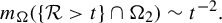 $$ \begin{align*}m_{\Omega}(\{\mathcal R>t\}\cap\Omega_2)\sim t^{-2}.\end{align*} $$
Now suppose
 $\Pi (\omega )\in \Omega _4.$
Notice that
$\Pi (\omega )\in \Omega _4.$
Notice that
 $\Omega _4$
can be written as
$\Omega _4$
can be written as
 $$ \begin{align*}\Omega_4=\{b\in(0,1],a\in(1-b,1],{\alpha}\in(1-b,a),s\in[0,(ab)^{-1})\}.\end{align*} $$
We have
 $$ \begin{align*}m_{{\mathcal{W}}}(\{\omega\in {\mathcal{W}}_{\mathrm{sa}}|\mathcal R(\omega)>t, \Pi(\omega)\in \Omega_4\}) = 4 m_{\Omega}(\{(a,b,s,{\alpha})\in\Omega_4: (ab)^{-1}-s>t\}).\end{align*} $$
The condition on the return time says
 $$ \begin{align*}(ab)^{-1}-s>t \iff (ab)^{-1}-t>s\end{align*} $$
and this is always the minimum upper bound for s in
 $\Omega _4$
since
$\Omega _4$
since
 $t>0$
. On the other hand, to satisfy the cross-term condition, we need
$t>0$
. On the other hand, to satisfy the cross-term condition, we need
 $$ \begin{align*}0<(ab)^{-1}-t \iff a<1/bt.\end{align*} $$
Hence, we are interested in the hyperbola
 $a =1/bt$
and how it intersects the triangle
$a =1/bt$
and how it intersects the triangle
 $\{b\in (0,1],a\in (1-b,1]\}.$
If
 $t\in [0,1)$
, then everything lies below the hyperbola
$t\in [0,1)$
, then everything lies below the hyperbola
 ${\alpha }={1}/{bt}$
and the contribution is
${\alpha }={1}/{bt}$
and the contribution is
 $$ \begin{align*}m_{\Omega}(\{\mathcal R>t\}\cap\Omega_4)=\int _{b=0} ^{1} \int_{a=1-b} ^{1} \int_{{\alpha}=1-b} ^ a \int _{s=0} ^{(ab)^{-1}-t} 1\,ds\,da\,d{\alpha}\,db.\end{align*} $$
If
 $t\in [1,4)$
, then the hyperbola
$t\in [1,4)$
, then the hyperbola
 ${\alpha }={1}/{bt}$
intersects once at
${\alpha }={1}/{bt}$
intersects once at
 $b=1/t$
and the integral is
$b=1/t$
and the integral is
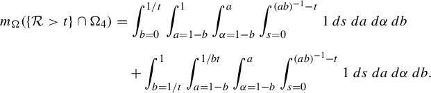 $$ \begin{align*} m_{\Omega}(\{\mathcal R>t\}\cap\Omega_4)&= \int _{b=0} ^{1/t} \int_{a=1-b} ^{1} \int_{{\alpha}=1-b} ^ a \int _{s=0} ^{(ab)^{-1}-t} 1\,ds\,da\,d{\alpha}\,db \\[5pt] &\quad+ \int _{b=1/t} ^{1} \int_{a=1-b} ^{1/bt} \int_{{\alpha}=1-b} ^ a \int _{s=0} ^{(ab)^{-1}-t} 1\,ds\,da\,d{\alpha}\,db. \end{align*} $$
If
 $t\in [4,\infty )$
, then the hyperbola
$t\in [4,\infty )$
, then the hyperbola
 ${\alpha }={1}/{bt}$
intersects twice and the integral is
${\alpha }={1}/{bt}$
intersects twice and the integral is
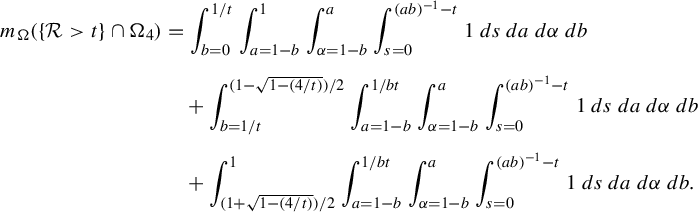 $$ \begin{align*} m_{\Omega}(\{\mathcal R>t\}\cap\Omega_4)& =\int_{b=0}^{1/t}\int_{a=1-b}^{1} \int_{{\alpha}=1-b} ^ a \int _{s=0} ^{(ab)^{-1}-t} 1\,ds\,da\,d{\alpha}\,db \\[5pt] &\quad+ \int _{b=1/t} ^{({1-\sqrt{1-(4/t)}})/{2}} \int_{a=1-b} ^{1/bt} \int_{{\alpha}=1-b} ^ a \int _{s=0} ^{(ab)^{-1}-t} 1\,ds\,da\,d{\alpha}\,db \\[5pt] &\quad+ \int _{({1+\sqrt{1-(4/t)}})/{2}}^1 \int_{a=1-b} ^{1/bt} \int_{{\alpha}=1-b} ^ a \int _{s=0} ^{(ab)^{-1}-t} 1\,ds\,da\,d{\alpha}\,db. \end{align*} $$
By evaluating each integral and approximating the result with a Taylor series, we see that
 $$ \begin{align*} \int_{b=0}^{1/t}\int_{a=1-b}^{1} \int_{{\alpha}=1-b} ^ a \int _{s=0} ^{(ab)^{-1}-t} 1\,ds\,da\,d{\alpha}\,db \sim t^{-2},\quad \ \ \ \ \ \\[5pt] \int _{b=1/t} ^{({1-\sqrt{1-(4/t)}})/{2}} \int_{a=1-b} ^{1/bt} \int_{{\alpha}=1-b} ^ a \int _{s=0} ^{(ab)^{-1}-t} 1\,ds\,da\,d{\alpha}\,db \sim t^{-4},\\[5pt] \int _{({1+\sqrt{1-(4/t)}})/{2}}^1 \int_{a=1-b} ^{1/bt} \int_{{\alpha}=1-b} ^ a \int _{s=0} ^{(ab)^{-1}-t} 1\,ds\,da\,d{\alpha}\,db \sim t^{-2}, \ \end{align*} $$
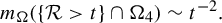 $$ \begin{align*}m_{\Omega}(\{\mathcal R>t\}\cap\Omega_4)\sim t^{-2}. \end{align*} $$
Tail contribution of
 ${\mathcal {W}}_{\mathrm{sa}} $
. Hence, combining all the above contributions, we have that the tail on
${\mathcal {W}}_{\mathrm{sa}} $
. Hence, combining all the above contributions, we have that the tail on
 ${\mathcal {W}}_{\mathrm{sa}}$
has quadratic decay,
${\mathcal {W}}_{\mathrm{sa}}$
has quadratic decay,
 $$ \begin{align*}m_{{\mathcal{W}}}(\{\omega\in {\mathcal{W}}_{\mathrm{sa}}:\mathcal R(\omega)>t\})\sim t^{-2}.\end{align*} $$
A.1.2 Haar-measure computations and estimates for
${\mathcal {W}}_{\mathrm{sl}}$

We now compute the contribution on the doubled slit tori coming from a short lattice piece. That is,
 $$ \begin{align*}m_{\mathcal W}(\{\omega\in {\mathcal{W}}_{\mathrm{sl}}| \mathcal R(\omega)>t\}).\end{align*} $$
For
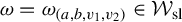 $\omega =\omega _{(a,b,v_1,v_2)}\in {\mathcal {W}}_{\mathrm{sl}}$
, we have a piecewise map on two pieces depending on the length of
$\omega =\omega _{(a,b,v_1,v_2)}\in {\mathcal {W}}_{\mathrm{sl}}$
, we have a piecewise map on two pieces depending on the length of
 $b+v_1$
. In each piece, we know explicitly the return map and thus can compute
$b+v_1$
. In each piece, we know explicitly the return map and thus can compute
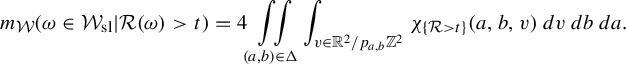 $$ \begin{align*}m_{{\mathcal{W}}}(\omega\in {\mathcal{W}}_{\mathrm{sl}}|\mathcal R(\omega)>t)= 4 \iint\limits_{(a,b)\in\Delta}\int_{v\in {\mathbb{R}}^2/p_{a,b}{\mathbb{Z}}^2}\chi_{\{ \mathcal R>t\}}(a,b,v)\,dv \,db \,da.\end{align*} $$
It will be useful to parameterize
 ${\mathbb {R}}^2/p_{a,b}{\mathbb {Z}}^2$
as the set
${\mathbb {R}}^2/p_{a,b}{\mathbb {Z}}^2$
as the set
 $$ \begin{align*}\{(v_1,v_2)=(ax+by,a^{-1}y)\mid (a,b)\in\Delta,(x,y)\in[0,1)^2\}.\end{align*} $$
The condition that determines what the return map is depends on whether
 $b+v_1$
is larger than or smaller than 1. In the coordinates
$b+v_1$
is larger than or smaller than 1. In the coordinates
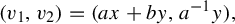 $(v_1,v_2)=(ax+by,a^{-1}y),$
we have
$(v_1,v_2)=(ax+by,a^{-1}y),$
we have
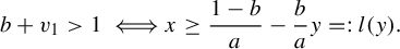 $$ \begin{align*}b+v_1>1\iff x\ge \frac{1-b}{a}-\frac{b}{a}y=:l(y).\end{align*} $$
Hence, there is natural interest in the behavior of l. Notice
-
(1)
$l(0)=({1-b})/{a} $
is always less than one for any
$(a,b)\in \Delta$
, and -
(2)
$l(1)<0\iff b>1/2$
.
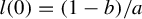


Hence, we can represent the two cases of our return map through the
 $(y,x)$
slice as in Figure A2.
$(y,x)$
slice as in Figure A2.
A generic picture of the two cases that arise for the return map.
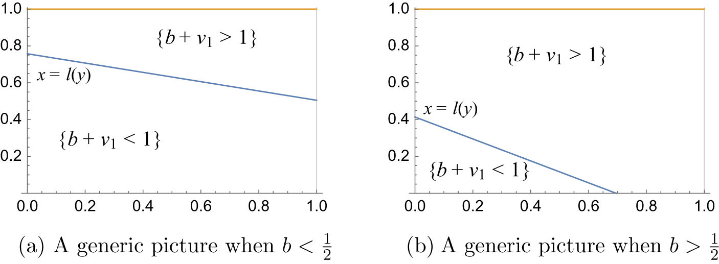
Case 1:
 $b+v_1>1$
. Notice that
$b+v_1>1$
. Notice that
 $l(1)<0\iff b>1/2$
. Moreover, l hits the y-axis at
$l(1)<0\iff b>1/2$
. Moreover, l hits the y-axis at
 $y=b^{-1}-1.$
As indicated at the start of this subsection, we break our computation up into the case where
$y=b^{-1}-1.$
As indicated at the start of this subsection, we break our computation up into the case where
 $b>1/2$
and
$b>1/2$
and
 $b<1/2$
. Notice that l hits the y-axis at
$b<1/2$
. Notice that l hits the y-axis at
 $y=b^{-1}-1$
.
$y=b^{-1}-1$
.
Case 1A:
 $b+v_1>1$
and
$b+v_1>1$
and
 $b<1/2$
. If
$b<1/2$
. If
 $b<1/2$
, then our region
$b<1/2$
, then our region
 $b+v_1>1$
can be described as
$b+v_1>1$
can be described as
 $$ \begin{align*}\{(b,a,x,y)\mid b\in(0,1/2],a\in(1-b,1),y\in[0,1),x\in[l(y),1)\}.\end{align*} $$
See Figure A2(a).
On this region,
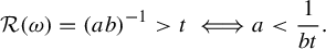 $$ \begin{align*}\mathcal R(\omega)=(ab)^{-1}>t\iff a<\frac{1}{bt}.\end{align*} $$
Hence, all we have to do is understand how this hyperbola intersects the triangle
 $\{(b,a)\in \Delta :b\in (1,1/2),a\in (1-b,1)\}$
.
$\{(b,a)\in \Delta :b\in (1,1/2),a\in (1-b,1)\}$
.
If
 $t\in [0,2)$
, then everything lies below the hyperbola and the contribution is given by
$t\in [0,2)$
, then everything lies below the hyperbola and the contribution is given by
 $$ \begin{align*}\int_{b=0} ^{1/2} \int_{a=1-b} ^1 \int _{y=0} ^{1} \int_{x=l(y)} ^1 1\,dx\,dy\,da\,db.\end{align*} $$
If
 $t\in [2,4)$
, then the contribution is given by
$t\in [2,4)$
, then the contribution is given by
 $$ \begin{align*}\int_{b=0} ^{1/t} \int_{a=1-b} ^1 \int _{y=0} ^{1} \int_{x=l(y)} ^1 1\,dx\,dy\,da\,db +\int_{b=1/t} ^{1/2} \int_{a=1-b} ^{1/bt} \int _{y=0} ^{1} \int_{x=l(y)} ^1 1\,dx\,dy\,da\,db.\end{align*} $$
If
 $t\in [4,\infty )$
, then the contribution is given by
$t\in [4,\infty )$
, then the contribution is given by
 $$ \begin{align*}&\int_{b=0} ^{1/t} \int_{a=1-b} ^{1} \int _{y=0} ^{1} \int_{x=l(y)} ^1 1\,dx\,dy\,da\,db\\ &\quad+\int_{b=1/t} ^{({1-\sqrt{1-(4/t)}})/{2}} \int_{a=1-b} ^{1/bt} \int _{y=0} ^{1} \int_{x=l(y)} ^1 1\,dx\,dy\,da\,db. \end{align*} $$
By evaluating each integral and approximating the result with a Taylor series, we see that
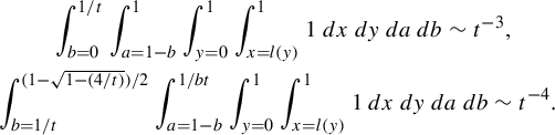 $$ \begin{align*} \int_{b=0} ^{1/t} \int_{a=1-b} ^{1} \int _{y=0} ^{1} \int_{x=l(y)} ^1 1\,dx\,dy\,da\,db \sim t^{-3},\qquad \\ \int_{b=1/t} ^{({1-\sqrt{1-(4/t)}})/{2}} \int_{a=1-b} ^{1/bt} \int _{y=0} ^{1} \int_{x=l(y)} ^1 1\,dx\,dy\,da\,db\sim t^{-4}. \end{align*} $$
Hence, the tail on this region is less than quadratic. More precisely, we have
 $$ \begin{align*}m_{{\mathcal{W}}}(\{\mathcal R>t\}\cap\{b+v_1>1\}\cap\{b<1/2\}) \sim t^{-3}.\end{align*} $$
Case 1B:
 $b+v_1>1$
and
$b+v_1>1$
and
 $b>1/2$
. If
$b>1/2$
. If
 $b>1/2$
, then our region is the union of
$b>1/2$
, then our region is the union of
 $$ \begin{align*}\{(b,a,x,y)\mid b\in(1/2,1),a\in(1-b,1),y\in[0,b^{-1}-1),x\in[l(y),1)\}\end{align*} $$
with
 $$ \begin{align*}\{(b,a,x,y)\mid b\in(1/2,1),a\in(1-b,1),y\in[b^{-1}-1,1),x\in[0,1)\}.\end{align*} $$
See Figure A2(b).
Now we can implement the return time condition. On this region,
 $$ \begin{align*}R(\omega)=(ab)^{-1}>t\iff (bt)^{-1}>a.\end{align*} $$
Hence, all we have to do is understand how this hyperbola intersects the triangle
 $\{(b,a)\in \Delta \mid b\in (1/2,1),a\in (1-b,1)\}$
.
$\{(b,a)\in \Delta \mid b\in (1/2,1),a\in (1-b,1)\}$
.
If
 $t\in (0,1)$
, then everything lies below the hyperbola and the integral is
$t\in (0,1)$
, then everything lies below the hyperbola and the integral is
 $$ \begin{align*}\int_{b=1/2} ^1 \int_{a=1-b} ^1 \bigg[\int _{y=0} ^{b^{-1}-1} \int_{x=l(y)} ^1 1\,dx\,dy + \int _{y=b^{-1}-1} ^{1} \int_{x=0} ^1 1\,dx\,dy \bigg] \,da\,db.\end{align*} $$
If
 $t\in [1,2)$
, then the integral is
$t\in [1,2)$
, then the integral is
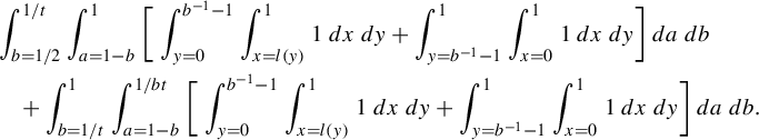 $$ \begin{align*} &\int_{b=1/2} ^{1/t} \int_{a=1-b} ^1 \bigg[\int _{y=0} ^{b^{-1}-1} \int_{x=l(y)} ^1 1\,dx\,dy + \int _{y=b^{-1}-1} ^{1} \int_{x=0} ^1 1\,dx\,dy \bigg] \,da\,db \\ &\quad+\int_{b=1/t} ^{1} \int_{a=1-b} ^{1/bt} \bigg[\int _{y=0} ^{b^{-1}-1} \int_{x=l(y)} ^1 1\,dx\,dy + \int _{y=b^{-1}-1} ^{1} \int_{x=0} ^1 1\,dx\,dy \bigg] \,da\,db. \end{align*} $$
If
 $t\in [2,4)$
, then the integral is
$t\in [2,4)$
, then the integral is
 $$ \begin{align*}\int_{b=1/2} ^{1} \int_{a=1-b} ^{1/bt} \bigg[\int _{y=0} ^{b^{-1}-1} \int_{x=l(y)} ^1 1\,dx\,dy + \int _{y=b^{-1}-1} ^{1} \int_{x=0} ^1 1\,dx\,dy \bigg] \,da\,db.\end{align*} $$
If
 $t\in [4,\infty )$
, then the integral is
$t\in [4,\infty )$
, then the integral is
 $$ \begin{align*}\int_{b=({1+\sqrt{1-(4/t)}})/{2}} ^{1} \int_{a=1-b} ^{1/bt} \bigg[\int _{y=0} ^{b^{-1}-1} \int_{x=l(y)} ^1 1\,dx\,dy + \int _{y=b^{-1}-1} ^{1} \int_{x=0} ^1 1\,dx\,dy \bigg] \,da\,db.\end{align*} $$
By evaluating this integral and approximating the result with a Taylor series, we see that
 $$ \begin{align*}\int_{b=({1+\sqrt{1-(4/t)}})/{2}} ^{1} \int_{a=1-b} ^{1/bt} \bigg[\!\int _{y=0} ^{b^{-1\kern-0.5pt}-1} \!\int_{x=l(y)} ^1 \!1\,dx\,dy \kern1pt{+}\kern1pt \int _{y=b^{-1\kern-0.5pt}-1} ^{1} \int_{x=0} ^1\! 1\,dx\,dy \!\bigg] da\,db \kern1pt{\sim}\kern1pt t^{\kern-0.5pt-2}.\end{align*} $$
Hence,
 $$ \begin{align*}m_{{\mathcal{W}}}(\{\mathcal R>t\}\cap\{b+v_1>1\}\cap\{b>1/2\})\end{align*} $$
decays quadratically.
Combining this with the part where
 $b<1/2$
, we see that
$b<1/2$
, we see that
 $$ \begin{align*}m_{{\mathcal{W}}}(\{\mathcal R>t\}\cap\{b+v_1>1\}) \sim t^{-2}.\end{align*} $$
Case 2:
 $b+v_1 <1$
. We are interested in the situation underneath
$b+v_1 <1$
. We are interested in the situation underneath
 $l(y)$
in Figure A2. Now we impose the return time condition. On this region (that is, when
$l(y)$
in Figure A2. Now we impose the return time condition. On this region (that is, when
 $b+v_1\le 1$
), we have
$b+v_1\le 1$
), we have
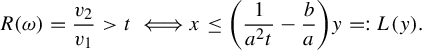 $$ \begin{align*}R(\omega) = \frac{v_2}{v_1}>t\iff x \le \bigg(\frac{1}{a^2t}-\frac{b}{a}\bigg)y=:L(y).\end{align*} $$
Notice that L is a line through the origin and since it is an upper bound for x, then we are only concerned when it has positive slope. That is, when
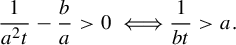 $$ \begin{align*}\frac{1}{a^2t}-\frac{b}{a}>0\iff \frac{1}{bt}>a.\end{align*} $$
Lastly, we notice to parameterize the
 $(y,x)$
-plane, we need to understand how the two lines l and L intersect each other. Since they are each lines, it suffices to understand how they interact when
$(y,x)$
-plane, we need to understand how the two lines l and L intersect each other. Since they are each lines, it suffices to understand how they interact when
 $y=1.$
We obtain three cases:
$y=1.$
We obtain three cases:
-
(1)
$b>1/2$
and
$L(1)\ge l(1);$
-
(2)
$b<1/2$
and
$L(1)\ge l(1);$
-
(3)
$b<1/2$
and
$L(1)< l(1).$


We do not have the case
 $b>1/2$
and
$b>1/2$
and
 $L(1)< l(1)$
because when
$L(1)< l(1)$
because when
 $b>1/2$
, then we have
$b>1/2$
, then we have
 $l(1)$
as negative, which forces L to be negative, but this is not possible since it is an upper bound for x. Lastly, we note that L and l intersect at the point
$l(1)$
as negative, which forces L to be negative, but this is not possible since it is an upper bound for x. Lastly, we note that L and l intersect at the point
 $y=(1-b)at.$
We illustrate the three cases in Figure A3.
$y=(1-b)at.$
We illustrate the three cases in Figure A3.
A generic picture of the three cases that arise for the return map.
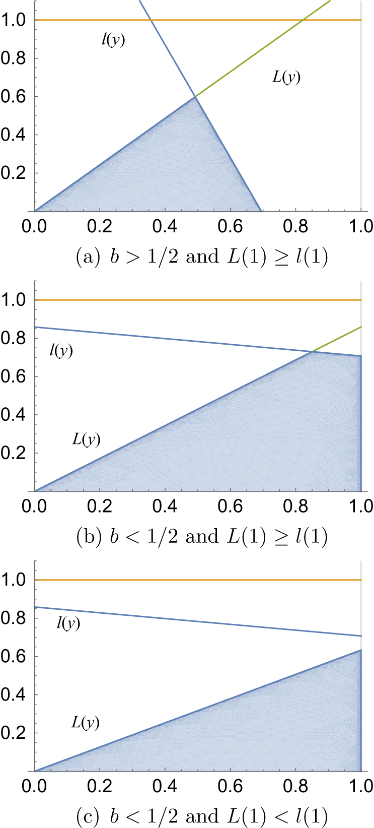
We now compute the contribution on each of the above cases.
Case 2A:
 $b+v_1 <1$
,
$b+v_1 <1$
,
 $b>1/2$
, and
$b>1/2$
, and
 $L(1)\ge l(1)$
. If
$L(1)\ge l(1)$
. If
 $b>1/2$
and
$b>1/2$
and
 $L(1)\ge l(1)$
, then the region is the union of
$L(1)\ge l(1)$
, then the region is the union of
 $$ \begin{align*}\{(b,a,y,x): b\in(1/2,1], a\in(1-b,1],y\in(0,(1-b)at],x\in(0,L(y))\}\end{align*} $$
and
 $$ \begin{align*}\{(b,a,y,x): b\in(1/2,1], a\in(1-b,1],y\in((1-b)at,b^{-1}-1],x\in(0,l(y))\}.\end{align*} $$
The condition
 $L(1)\ge l(1)$
is equivalent to
$L(1)\ge l(1)$
is equivalent to
 $a\le {1}/{t(1-b)}$
. Combining this with the condition from the return map means that we are interested in
$a\le {1}/{t(1-b)}$
. Combining this with the condition from the return map means that we are interested in
 $$ \begin{align*}a\le\min\bigg\{\frac{1}{bt},\frac{1}{t(1-b)}\bigg\}.\end{align*} $$
However,
 $$ \begin{align*}\frac{1}{tb}<\frac{1}{t(1-b)}\iff1/2<b\end{align*} $$
so that actually we only care about how the hyperbola
 $a={1}/{tb}$
intersects the region
$a={1}/{tb}$
intersects the region
 $\{(b,a):b\in (1/2,1],a\in (1-b,1]\}.$
If
 $t\in [0,1)$
, then everything is under the hyperbola and the integral is
$t\in [0,1)$
, then everything is under the hyperbola and the integral is
 $$ \begin{align*}\int_{b=1/2} ^{1}\int_{a=1-b}^{1} \bigg[ \int_{y=0} ^{(1-b)at} \int_{x=0} ^{L(y)} 1\,dx\,dy + \int_{y=(1-b)at} ^{b^{-1}-1} \int_{x=0} ^{l(y)} 1\,dx\,dy \bigg]\,da\,db.\end{align*} $$
If
 $t\in [1,2)$
, then the integral is
$t\in [1,2)$
, then the integral is
 $$ \begin{align*} &\int_{b=1/2} ^{1/t}\int_{a=1-b}^{1} \bigg[ \int_{y=0} ^{(1-b)at} \int_{x=0} ^{L(y)} 1\,dx\,dy + \int_{y=(1-b)at} ^{b^{-1}-1} \int_{x=0} ^{l(y)} 1\,dx\,dy \bigg]\,da\,db\\ &\quad+\int_{b=1/t} ^{1}\int_{a=1-b}^{1/bt} \bigg[ \int_{y=0} ^{(1-b)at} \int_{x=0} ^{L(y)} 1\,dx\,dy + \int_{y=(1-b)at} ^{b^{-1}-1} \int_{x=0} ^{l(y)} 1\,dx\,dy \bigg]\,da\,db. \end{align*} $$
If
 $t\in [2,4)$
, then the integral is
$t\in [2,4)$
, then the integral is
 $$ \begin{align*} \int_{b=1/2} ^{1}\int_{a=1-b}^{1/bt} \bigg[ \int_{y=0} ^{(1-b)at} \int_{x=0} ^{L(y)} 1\,dx\,dy + \int_{y=(1-b)at} ^{b^{-1}-1} \int_{x=0} ^{l(y)} 1\,dx\,dy \bigg]\,da\,db. \end{align*} $$
If
 $t\in [4,\infty )$
, then the integral is
$t\in [4,\infty )$
, then the integral is
 $$ \begin{align*} \int_{b=({1+\sqrt{1-(4/t)}})/{2}} ^{1}\int_{a=1-b}^{1/bt} \bigg[ \int_{y=0} ^{(1-b)at} \int_{x=0} ^{L(y)} 1\,dx\,dy + \int_{y=(1-b)at} ^{b^{-1}-1} \int_{x=0} ^{l(y)} 1\,dx\,dy \bigg]\,da\,db. \end{align*} $$
By evaluating the above integral and approximating it with its Taylor series we see that the decay is cubic. That is,
 $$ \begin{align*}m_{{\mathcal{W}}}(\{\mathcal R>t\}\cap\{b+v_1<1\}\cap\{b>1/2\} \cap\{L(1)\ge l(1)\} ) \sim t^{-3}.\end{align*} $$
Case 2B:
 $b+v_1 <1$
,
$b+v_1 <1$
,
 $b<1/2$
, and
$b<1/2$
, and
 $L(1)\ge l(1)$
. If
$L(1)\ge l(1)$
. If
 $b<1/2$
and
$b<1/2$
and
 $L(1)\ge l(1)$
, then the region is the union of
$L(1)\ge l(1)$
, then the region is the union of
 $$ \begin{align*}\{(b,a,y,x): b\in(0,1/2], a\in(1-b,1],y\in(0,(1-b)at],x\in(0,L(y))\}\end{align*} $$
and
 $$ \begin{align*}\{(b,a,y,x): b\in(0,1/2], a\in(1-b,1],y\in((1-b)at,1],x\in(0,l(y))\}.\end{align*} $$
As before, the condition
 $L(1)\ge l(1)$
is equivalent to
$L(1)\ge l(1)$
is equivalent to
 $a\le {1}/{t(1-b)}$
. Combining this with the condition from the return map means that we are interested in
$a\le {1}/{t(1-b)}$
. Combining this with the condition from the return map means that we are interested in
 $$ \begin{align*}a\le\min\bigg\{\frac{1}{bt},\frac{1}{t(1-b)}\bigg\}.\end{align*} $$
We have,
 $$ \begin{align*}\frac{1}{tb}>\frac{1}{t(1-b)}\iff1/2>b.\end{align*} $$
Consequently, we are interested in how the hyperbola
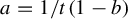 $a={1}/{t(1-b)}$
intersects the triangle
$a={1}/{t(1-b)}$
intersects the triangle
 $\{(b,a):b\in (0,1/2],a\in (1-b,1]\}$
.
$\{(b,a):b\in (0,1/2],a\in (1-b,1]\}$
.
If
 $t\in [0,1)$
, then everything is under the hyperbola and the integral is
$t\in [0,1)$
, then everything is under the hyperbola and the integral is
 $$ \begin{align*}\int_{b=0} ^{1/2}\int_{a=1-b}^{1} \bigg[ \int_{y=0} ^{(1-b)at} \int_{x=0} ^{L(y)} 1\,dx\,dy + \int_{y=(1-b)at} ^{1} \int_{x=0} ^{l(y)} 1\,dx\,dy \bigg]\,da\,db.\end{align*} $$
If
 $t\in [1,2)$
, then the integral is
$t\in [1,2)$
, then the integral is
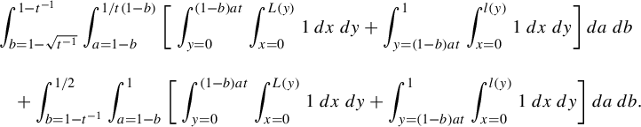 $$ \begin{align*} &\int_{b=1-\sqrt{t^{-1}}} ^{1-t^{-1}}\int_{a=1-b}^{{1}/{t(1-b)}} \bigg[ \int_{y=0} ^{(1-b)at} \int_{x=0} ^{L(y)} 1\,dx\,dy + \int_{y=(1-b)at} ^{1} \int_{x=0} ^{l(y)} 1\,dx\,dy \bigg]\,da\,db\\ &\quad+\int_{b=1-t^{-1}} ^{1/2}\int_{a=1-b}^{1} \bigg[ \int_{y=0} ^{(1-b)at} \int_{x=0} ^{L(y)} 1\,dx\,dy + \int_{y=(1-b)at} ^{1} \int_{x=0} ^{l(y)} 1\,dx\,dy \bigg]\,da\,db. \end{align*} $$
If
 $t\in [2,4)$
, then the integral is
$t\in [2,4)$
, then the integral is
 $$ \begin{align*} \int_{b=1-\sqrt{t^{-1}}} ^{1/2}\int_{a=1-b}^{{1}/{t(1-b)}} \bigg[ \int_{y=0} ^{(1-b)at} \int_{x=0} ^{L(y)} 1\,dx\,dy + \int_{y=(1-b)at} ^{1} \int_{x=0} ^{l(y)} 1\,dx\,dy \bigg]\,da\,db. \end{align*} $$
If
 $t\in [4,\infty )$
, then the hyperbola passes below the triangle and there is no contribution.
$t\in [4,\infty )$
, then the hyperbola passes below the triangle and there is no contribution.
Case 2C:
 $b+v_1 <1$
,
$b+v_1 <1$
,
 $b<1/2$
, and
$b<1/2$
, and
 $L(1)< l(1)$
. If
$L(1)< l(1)$
. If
 $b<1/2$
and
$b<1/2$
and
 $L(1)< l(1)$
, then the region is
$L(1)< l(1)$
, then the region is
 $$ \begin{align*}\{(b,a,y,x): b\in(0,1/2], a\in(1-b,1],y\in(0,1],x\in(0,L(y))\}.\end{align*} $$
Using that
 $L(1)<l(1)$
is equivalent to
$L(1)<l(1)$
is equivalent to
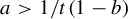 $a>{1}/{t(1-b)}$
. we have that we are interested in the condition:
$a>{1}/{t(1-b)}$
. we have that we are interested in the condition:
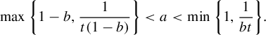 $$ \begin{align*}\max\bigg\{1-b,\frac{1}{t(1-b)}\bigg\}<a<\min\bigg\{1,\frac{1}{bt}\bigg\}.\end{align*} $$
By understanding this region in the
 $(b,a)$
-slice we deduce the following.
$(b,a)$
-slice we deduce the following.
If
 $t\in [0,1)$
, the condition that
$t\in [0,1)$
, the condition that
 $a>{1}/{t(1-b)}$
says there is no contribution here.
$a>{1}/{t(1-b)}$
says there is no contribution here.
If
 $t\in [1,2)$
, the integral is
$t\in [1,2)$
, the integral is
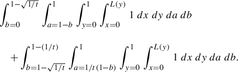 $$ \begin{align*}&\int_{b=0} ^{1-\sqrt{1/t}}\int_{a=1-b}^{1} \int_{y=0} ^{1} \int_{x=0} ^{L(y)} 1\,dx\,dy \,da\,db\\ &\quad+ \int_{b=1-\sqrt{1/t}} ^{1-(1/t)}\int_{a={1}/{t(1-b)}}^{1} \int_{y=0} ^{1} \int_{x=0} ^{L(y)} 1\,dx\,dy \,da\,db.\end{align*} $$
If
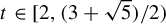 $t\in [2,({3+\sqrt {5}})/{2})$
, the integral is
$t\in [2,({3+\sqrt {5}})/{2})$
, the integral is
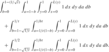 $$ \begin{align*} &\int_{b=0} ^{1-({1}/{\sqrt{t}})}\int_{a=1-b}^{1} \int_{y=0} ^{1} \int_{x=0} ^{L(y)} 1\,dx\,dy \,da\,db \\ &\quad+ \int_{b=1-\sqrt{1/t}} ^{1/t}\int_{a={1}/{t(1-b)}}^{1/bt} \int_{y=0} ^{1} \int_{x=0} ^{L(y)} 1\,dx\,dy \,da\,db \\ &\quad+ \int_{b=1-\sqrt{1/t}} ^{1/2} \int_{a={1}/{t(1-b)}}^{1/bt} \int_{y=0} ^{1} \int_{x=0} ^{L(y)} 1\,dx\,dy \,da\,db. \end{align*} $$
If
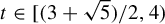 $t\in [({3+\sqrt {5}})/{2},4)$
, the integral is
$t\in [({3+\sqrt {5}})/{2},4)$
, the integral is
 $$ \begin{align*} &\int_{b=0} ^{1/t}\int_{a=1-b}^{1} \int_{y=0} ^{1} \int_{x=0} ^{L(y)} 1\,dx\,dy \,da\,db + \int_{b=1/t} ^{1-\sqrt{1/t}}\int_{a=1-b}^{1/bt} \int_{y=0} ^{1} \int_{x=0} ^{L(y)} 1\,dx\,dy \,da\,db \\ &\quad+ \int_{b=1-\sqrt{1/t}} ^{1/2} \int_{a={1}/{t(1-b)}}^{1/bt} \int_{y=0} ^{1} \int_{x=0} ^{L(y)} 1\,dx\,dy \,da\,db. \end{align*} $$
Lastly, if
 $t\ge 4$
, the integral is
$t\ge 4$
, the integral is
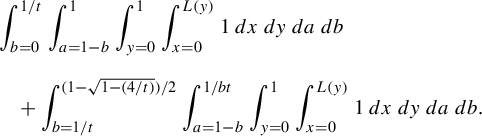 $$ \begin{align*}&\int_{b=0} ^{1/t}\int_{a=1-b}^{1} \int_{y=0} ^{1} \int_{x=0} ^{L(y)} 1\,dx\,dy \,da\,db\\ &\quad+ \int_{b=1/t} ^{({1-\sqrt{1-(4/t)}})/{2}}\int_{a=1-b}^{{1}/{bt}} \int_{y=0} ^{1} \int_{x=0} ^{L(y)} 1\,dx\,dy \,da\,db.\end{align*} $$
By evaluating the integrals and approximating it with its Taylor series we see that the decay is cubic.
A.1.3 Proof of Theorem 4.4, (3) and (4)
Combining the results of the previous two subsections we see that we have quadratic decay for the slope gap distribution of doubled slit tori and support at zero.
An explicit description of the tail distribution G is given below. Recall, that this is defined as
 $G(t)=\tfrac {1}{6} (3+\pi ^2)-F(t)$
where
$G(t)=\tfrac {1}{6} (3+\pi ^2)-F(t)$
where
 $F(t)$
is the cummulative distribution function.
$F(t)$
is the cummulative distribution function.
Piecewise, we have:
 $G(t) \cdot \chi _{[0,1]}=\tfrac {1}{6} (3+\pi ^2)-({7 t}/{8}),$
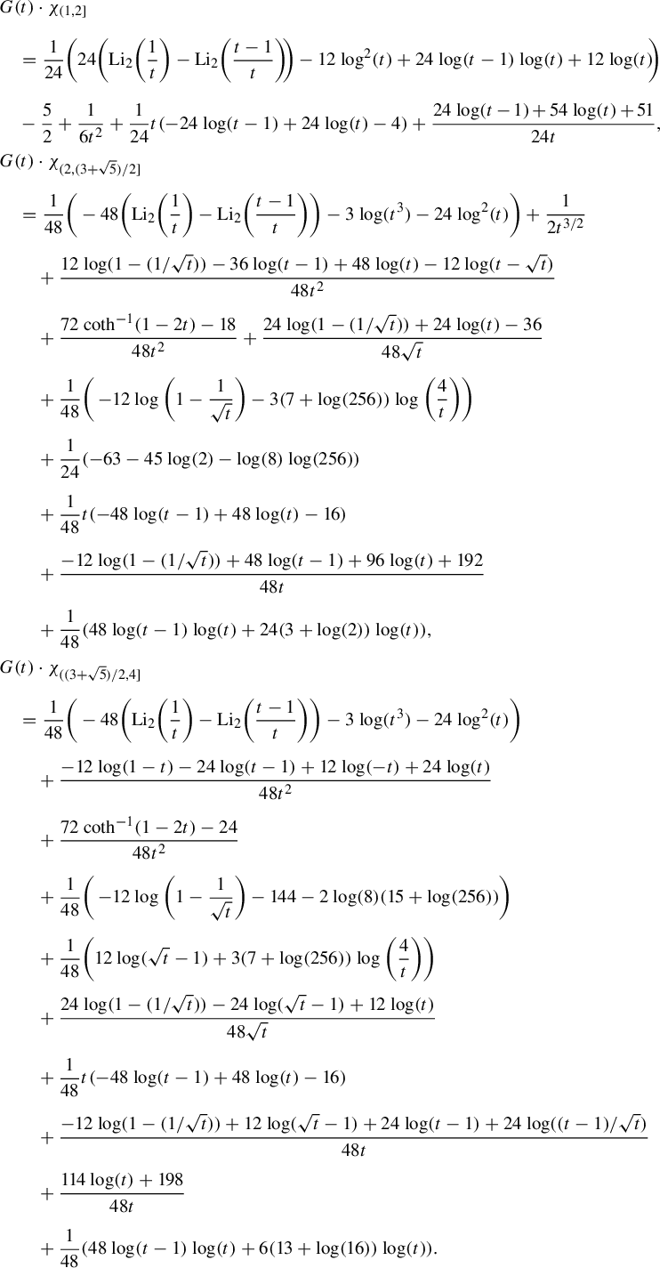 $$ \begin{align*} &G(t) \cdot \chi_{(1,2]}\\ &\quad=\frac{1}{24} \bigg(24 \bigg(\text{Li}_2\bigg(\frac{1}{t}\bigg)-\text{Li}_2\bigg(\frac{t-1}{t}\bigg)\!\bigg)-12 \log ^2(t)+24 \log (t-1) \log (t)+12 \log (t)\!\bigg)\\ &\quad-\frac{5}{2}+\frac{1}{6 t^2}+\frac{1}{24} t (-24 \log (t-1)+24 \log (t)-4)+\frac{24 \log (t\kern1.5pt{-}\kern1.5pt1)\kern1.5pt{+}\kern1.5pt54 \log (t)\kern1.5pt{+}\kern1.5pt 51}{24 t}, \\ &G(t) \cdot \chi_{(2,({3+\sqrt{5}})/{2}]}\\ &\quad=\frac{1}{48} \bigg(-48 \bigg(\text{Li}_2\bigg(\frac{1}{t}\bigg)-\text{Li}_2\bigg(\frac{t-1}{t}\bigg)\bigg)-3 \log (t^3)-24 \log ^2(t)\bigg)+\frac{1}{2 t^{3/2}}\\ &\qquad+\frac{12 \log (1-({1}/{\sqrt{t}}))-36 \log (t-1)+48 \log (t)-12 \log (t-\sqrt{t})}{48 t^2}\\ &\qquad+\frac{72 \coth ^{-1}(1-2 t)-18}{48 t^2}+\frac{24 \log (1-({1}/{\sqrt{t}}))+24 \log (t)-36}{48 \sqrt{t}}\\ &\qquad+\frac{1}{48} \bigg(-\!12 \log \bigg(1-\frac{1}{\sqrt{t}}\bigg)-3 (7+\log (256)) \log \bigg(\frac{4}{t}\bigg)\bigg)\\ &\qquad+\frac{1}{24} (-63-45 \log (2)-\log (8) \log (256))\\ &\qquad+\frac{1}{48} t (-48 \log (t-1)+48 \log (t)-16)\\ &\qquad+\frac{-12 \log (1-({1}/{\sqrt{t}}))+48 \log (t-1)+96 \log (t)+192}{48 t}\\ &\qquad+\frac{1}{48} (48 \log (t-1) \log (t)+24 (3+\log (2)) \log (t)), \\ &G(t) \cdot \chi_{(({3+\sqrt{5}})/{2},4]}\\ &\quad=\frac{1}{48} \bigg(-48 \bigg(\text{Li}_2\bigg(\frac{1}{t}\bigg)-\text{Li}_2\bigg(\frac{t-1}{t}\bigg)\bigg)-3 \log (t^3)-24 \log ^2(t)\bigg)\\ &\qquad+\frac{-12 \log (1-t)-24 \log (t-1)+12 \log (-t)+24 \log (t)}{{48 t^2}}\\ &\qquad+\frac{72 \coth ^{-1}(1-2 t)-24}{48 t^2}\\ &\qquad+\frac{1}{48} \bigg(-\!12 \log \bigg(1-\frac{1}{\sqrt{t}}\bigg)-144-2 \log (8) (15+\log (256))\bigg)\\ &\qquad+\frac{1}{48} \bigg(12 \log (\sqrt{t}-1)+3 (7+\log (256)) \log \bigg(\frac{4}{t}\bigg)\bigg)\\ &\qquad+\frac{24 \log (1-({1}/{\sqrt{t}}))-24 \log (\sqrt{t}-1)+12 \log (t)}{48 \sqrt{t}}\\ &\qquad+\frac{1}{48} t (-48 \log (t-1)+48 \log (t)-16)\\ &\qquad+\frac{-12 \log (1-({1}/{\sqrt{t}}))+12 \log (\sqrt{t}-1)+24 \log (t-1)+24 \log (({t-1})/{\sqrt{t}})}{48 t}\\ &\qquad+\frac{114 \log (t)+198}{48 t}\\ &\qquad+\frac{1}{48} (48 \log (t-1) \log (t)+6 (13+\log (16)) \log (t)). \end{align*} $$
The formula for
 $G(t)$
when
$G(t)$
when
 $t>4$
is extremely long so we do not write them down. The main characteristic is that it has quadratic tail decay as shown in Theorem 4.4(3).
$t>4$
is extremely long so we do not write them down. The main characteristic is that it has quadratic tail decay as shown in Theorem 4.4(3).
A.2 Haar measure computations and estimates for
$\Omega $

We prove the estimate of Theorem 4.4(1). We also show that there is support at zero for the density function.
Proof Proof of Theorem 4.4(1)
We compute the cumulative distribution function for the gaps of slopes
 $$ \begin{align*}m_{\Omega}(\{R>t\}\cap \Omega_i)\end{align*} $$
separately for each
 $i=1,\ldots ,4$
where
$i=1,\ldots ,4$
where
 $\Omega _i$
are the regions where the return map is the same.
$\Omega _i$
are the regions where the return map is the same.
We notice that much of these computations were needed in computing the gap distribution on
 ${\mathcal {W}}$
, specifically the ones for the tail of
${\mathcal {W}}$
, specifically the ones for the tail of
 $\Omega _1$
and
$\Omega _1$
and
 $\Omega _3$
. As such, we do not reproduce them here.
$\Omega _3$
. As such, we do not reproduce them here.
For
 $\Omega _1$
and
$\Omega _1$
and
 $\Omega _3$
we can compute exact asymptotics, while we only compute upper and lower bounds for
$\Omega _3$
we can compute exact asymptotics, while we only compute upper and lower bounds for
 $\Omega _2$
and
$\Omega _2$
and
 $\Omega _4$
. This is because the return time function includes a floor function in these cases which make explicit computations difficult.
$\Omega _4$
. This is because the return time function includes a floor function in these cases which make explicit computations difficult.
Tail on
 $\Omega _1$
. This computation was implicit in the section of measure estimates on
$\Omega _1$
. This computation was implicit in the section of measure estimates on
 ${\mathcal {W}}$
. It was shown there that for
${\mathcal {W}}$
. It was shown there that for
 $t>4$
, we have
$t>4$
, we have
 $$ \begin{align*}m_{\Omega}(\{R>t\}\cap \Omega_1) \sim t^{-2}.\end{align*} $$
Hence, the decay on
 $\Omega _1$
is quadratic.
$\Omega _1$
is quadratic.
Tail in
 $\Omega _2$
. Due to the floor function in the formula for the return map on
$\Omega _2$
. Due to the floor function in the formula for the return map on
 $\Omega $
, we only compute lower and upper estimates on the decay. We first notice that
$\Omega $
, we only compute lower and upper estimates on the decay. We first notice that
 $\Omega _2$
can be written as
$\Omega _2$
can be written as
 $$ \begin{align*}\Omega_2=\bigg\{b\in(0,1],a\in(1-b,1],{\alpha}\in(a,1),s\in\bigg[(ab)^{-1}\bigg(\frac{{\alpha}-a}{{\alpha}}\bigg),(ab)^{-1}\bigg)\bigg\}.\end{align*} $$
We compute an upper bound for the contribution on
 $\Omega _2$
. Recall that
$\Omega _2$
. Recall that
 $j = \lfloor ({1+a-{\alpha }})/{b}\rfloor $
is in the formula for the return map on
$j = \lfloor ({1+a-{\alpha }})/{b}\rfloor $
is in the formula for the return map on
 $\Omega _2$
. An upper bound is found by
$\Omega _2$
. An upper bound is found by
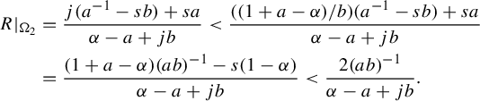 $$ \begin{align*} R|_{\Omega_2}&=\frac{j(a^{-1}-sb)+sa}{{\alpha}-a+jb}<\frac{(({1+a-{\alpha}})/{b})(a^{-1}-sb)+sa}{{\alpha}-a+jb}\\ &=\frac{(1+a-{\alpha})(ab)^{-1}-s(1-{\alpha})}{{\alpha}-a+jb}<\frac{2(ab)^{-1}}{{\alpha}-a+jb}. \end{align*} $$
Using that
 $$ \begin{align*}{\alpha}-a+jb>{\alpha}-a+\bigg(\frac{1+a-{\alpha}}{b}-1\bigg)b=1-b\end{align*} $$
and continuing our estimate from before, we find
 $$ \begin{align*}R|_{\Omega_2}<\frac{2(ab)^{-1}}{{\alpha}-a+jb}<\frac{2}{ab(1-b)}=:U.\end{align*} $$
To compute the contribution of
 $m_{\Omega }(\{t<U\})$
, we notice that
$m_{\Omega }(\{t<U\})$
, we notice that
 $$ \begin{align*}t<U\iff a<\frac{2}{tb(1-b)}.\end{align*} $$
Thus, we need to understand how the curve
 ${1}/{tb(1-b)}$
intersects the triangle
${1}/{tb(1-b)}$
intersects the triangle
 $\{(b,a): b\in (0,1], a\in (1-b,1]\} )$
. Due to this, the following points will be of interest
$\{(b,a): b\in (0,1], a\in (1-b,1]\} )$
. Due to this, the following points will be of interest
 $$ \begin{align*}b_k := \frac{2}{3}\bigg(\cos\bigg(\frac{1}{3}\arccos\bigg(\frac{54}{2t}-1\bigg)-\frac{2\pi *k}{3}\bigg)+1\bigg)\end{align*} $$
where
 $k=1,2.$
For t large, we note that
$k=1,2.$
For t large, we note that
 $b_1$
is close to 1 and
$b_1$
is close to 1 and
 $b_2$
is close to 0. These points correspond to where the curve
$b_2$
is close to 0. These points correspond to where the curve
 $a={1}/{tb(1-b)}$
intersects the line
$a={1}/{tb(1-b)}$
intersects the line
 $a=1-b$
.
$a=1-b$
.
Hence,
 $$ \begin{align*} m_{\Omega}(\{t<U\}) &= \int_{b=0} ^{({1-\sqrt{1-(8/t)}})/{2}} \int_{a=1-b} ^{1} \int_{{\alpha}=a} ^{1} \int _{s=({{\alpha}-a})/{ab{\alpha}}} ^{{1}/{ab}}1\,ds\,d{\alpha}\,da \,db\\[5pt] &\quad+ \int _{b={({1-\sqrt{1-(8/t)}})/{2}}} ^{b_2} \int_{a=1-b} ^{{1}/({bt(1-b)})} \int_{{\alpha}=a} ^ 1 \int _{s=({{\alpha}-a})/{ab{\alpha}}} ^{{1}/{ab}}1\,ds\,d{\alpha} \,da \,db\\[5pt] &\quad+ \int _{b=x_1} ^{({1+\sqrt{1-(8/t)}})/{2}} \int_{a=1-b} ^{{1}/({bt(1-b)})} \int_{{\alpha}=a} ^ 1 \int _{s=({{\alpha}-a})/{ab{\alpha}}} ^{{1}/{ab}}1\,ds\,d{\alpha}\,da \,db\\[5pt] &\quad+ \int _{b=({1+\sqrt{1-(8/t)}})/{2}} ^1 \int_{a=1-b} ^{1} \int_{{\alpha}=a} ^ 1 \int _{s=({{\alpha}-a})/{ab{\alpha}}} ^{{1}/{ab}}1\,ds\,d{\alpha}\,da \,db. \end{align*} $$
By evaluating each integral and approximating the result with a Taylor series, we see that
 $$ \begin{align*} \int_{b=0} ^{({1-\sqrt{1-(8/t)}})/{2}} \int_{a=1-b} ^{1} \int_{{\alpha}=a} ^{1} \int _{s=({{\alpha}-a})/{ab{\alpha}}} ^{{1}/{ab}}1\,ds\,d{\alpha}\,da \,db\sim t^{-2}, \quad \ \\[5pt] \int _{b={({1-\sqrt{1-(8/t)}})/{2}}} ^{b_2} \int_{a=1-b} ^{{1}/({bt(1-b)})} \int_{{\alpha}=a} ^ 1 \int _{s=({{\alpha}-a})/{ab{\alpha}}} ^{{1}/{ab}}1\,ds\,d{\alpha}\,da \,db\sim t^{-1},\\[5pt] \int _{b=b_1} ^{({1+\sqrt{1-(8/t)}})/{2}} \int_{a=1-b} ^{{1}/({bt(1-b)})} \int_{{\alpha}=a} ^ 1 \int _{s=({{\alpha}-a})/{ab{\alpha}}} ^{{1}/{ab}}1\,ds\,d{\alpha}\,da \,db\sim t^{-1}, \ \\[5pt] \int _{b=({1+\sqrt{1-(8/t)}})/{2}} ^1 \int_{a=1-b} ^{1} \int_{{\alpha}=a} ^ 1 \int _{s=({{\alpha}-a})/{ab{\alpha}}} ^{{1}/{ab}}1\,ds\,d{\alpha}\,da \,db\sim t^{-1}. \quad \end{align*} $$
Hence, an upper bound for the decay is
 $$ \begin{align*}m_{\Omega}(\{t<R\}\cap\Omega_2) <m_{\Omega}(\{t<U\}) \sim t^{-1}.\end{align*} $$
We now compute a lower bound for the contribution on
 $\Omega _2$
. Using that the denominator of R is bounded above by 1 and that all the terms in the numerator are positive, we have that
$\Omega _2$
. Using that the denominator of R is bounded above by 1 and that all the terms in the numerator are positive, we have that
 $$ \begin{align*}R|_{\Omega_2}=\frac{j(a^{-1}-sb)+sa}{{\alpha}-a+jb}>\frac{sa}{1}.\end{align*} $$
Finally, using the lower bound of s in
 $\Omega _2$
yields that
$\Omega _2$
yields that
 $$ \begin{align*}R|_{\Omega_2}>\frac{{\alpha}-a}{b{\alpha}}=:L.\end{align*} $$
To compute the contribution of
 $m_{\Omega }(\{t<L\})$
, we notice that
$m_{\Omega }(\{t<L\})$
, we notice that
 $$ \begin{align*}t<L\iff a<{\alpha}(1-bt),\end{align*} $$
which indicates interest in how the curve
 $a={\alpha }(1-bt)$
intersects the
$a={\alpha }(1-bt)$
intersects the
 $({\alpha },a)$
triangle. A computation confirms that we only have points in this triangle whenever
$({\alpha },a)$
triangle. A computation confirms that we only have points in this triangle whenever
 $b<1/t$
. Of those points, we only get a contribution whenever
$b<1/t$
. Of those points, we only get a contribution whenever
 $1-tb>1,$
which gives the integral
$1-tb>1,$
which gives the integral
 $$ \begin{align*}\int_{b=0} ^{1/t} \int_{{\alpha}=1-b} ^1 \int_{a=1-b} ^{\alpha} \int_{s=({{\alpha}-a})/{ab{\alpha}}} ^{(ab)^{-1}} 1\,ds\,da\,d{\alpha} \,db.\end{align*} $$
Evaluating and using Taylor series shows that this integral has quadratic decay that is
 $$ \begin{align*}\int_{b=0} ^{1/t} \int_{{\alpha}=1-b} ^1 \int_{a=1-b} ^{\alpha} \int_{s=({{\alpha}-a})/{ab{\alpha}}} ^{(ab)^{-1}} 1\,ds\,da\,d{\alpha} \,db\sim t^{-2}.\end{align*} $$
Tail on
 $\Omega _3$
. This computation was implicit in the section of measure estimates on
$\Omega _3$
. This computation was implicit in the section of measure estimates on
 ${\mathcal {W}}$
. It was shown there that for
${\mathcal {W}}$
. It was shown there that for
 $t>4$
, we have
$t>4$
, we have
 $$ \begin{align*}m_{\Omega}(\{R>t\}\cap \Omega_3) \sim t^{-2}.\end{align*} $$
Hence, the decay on
 $\Omega _3$
is quadratic.
$\Omega _3$
is quadratic.
Tail on
 $\Omega _4$
. We first notice that
$\Omega _4$
. We first notice that
 $\Omega _4$
can be written as
$\Omega _4$
can be written as
 $$ \begin{align*}\Omega_4 = \{b\in(0,1],a\in(1-b,1],{\alpha}\in(1-b,a], s\in[0,(ab)^{-1})\}.\end{align*} $$
Second, we notice that the upper estimate from
 $\Omega _2$
works. Namely,
$\Omega _2$
works. Namely,
 $$ \begin{align*}R|_{\Omega_4}< \frac{2}{ab(1-b)}=:U.\end{align*} $$
Moreover,
 $$ \begin{align*}t<U\iff a<\frac{2}{tb(1-b)}.\end{align*} $$
Thus, we need to understand how the curve
 ${1}/{tb(1-b)}$
intersects the triangle
${1}/{tb(1-b)}$
intersects the triangle
 $$ \begin{align*}\{(b,a): b\in(0,1], a\in(1-b,1]\} ).\end{align*} $$
As before, we will be interested in
 $$ \begin{align*}b_k := \frac{2}{3}\bigg(\cos\bigg(\frac{1}{3}\arccos\bigg(\frac{54}{2t}-1\bigg)-\frac{2\pi *k}{3}\bigg)+1\bigg),\end{align*} $$
where
 $k=1,2.$
For t large, we note that
$k=1,2.$
For t large, we note that
 $b_1$
is close to 1 and
$b_1$
is close to 1 and
 $b_2$
is close to 0. Lastly, these points correspond to where the curve
$b_2$
is close to 0. Lastly, these points correspond to where the curve
 $a={1}/{tb(1-b)}$
intersects the line
$a={1}/{tb(1-b)}$
intersects the line
 $a=1-b$
.
$a=1-b$
.
An upper bound for the contribution is given by
 $$ \begin{align*} m_{\Omega}(\{t<U\}) &= \int_{b=0} ^{({1-\sqrt{1-(8/t)}})/{2}} \int_{a=1-b} ^{1} \int_{{\alpha}=1-b} ^{a} \int _{s=0} ^{{1}/{ab}}1\,ds\,d{\alpha}\,da \,db\\ &\quad+ \int _{b={({1-\sqrt{1-(8/t)}})/{2}}} ^{b_2} \int_{a=1-b} ^{{1}/({bt(1-b)})} \int_{{\alpha}=1-b} ^{a} \int _{s=0} ^{{1}/{ab}}1\,ds\,d{\alpha}\,da \,db\\ &\quad+ \int _{b=b_1} ^{({1+\sqrt{1-(8/t)}})/{2}} \int_{a=1-b} ^{{1}/({bt(1-b)})} \int_{{\alpha}=1-b} ^{a} \int _{s=0} ^{{1}/{ab}}1\,ds\,d{\alpha}\,da \,db\\ &\quad+ \int _{b=({1+\sqrt{1-(8/t)}})/{2}} ^1 \int_{a=1-b} ^{1} \int_{{\alpha}=1-b} ^{a} \int _{s=0} ^{{1}/{ab}}1\,ds\,d{\alpha}\,da \,db. \end{align*} $$
We find the decay of each term to be
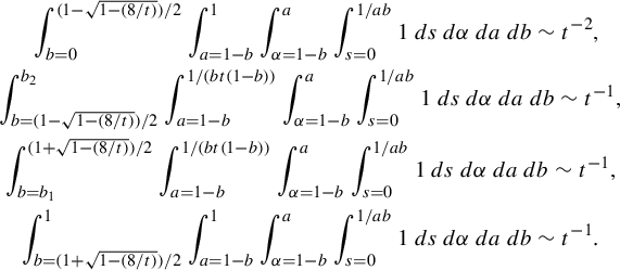 $$ \begin{align*} \int_{b=0} ^{({1-\sqrt{1-(8/t)}})/{2}} \int_{a=1-b} ^{1} \int_{{\alpha}=1-b} ^{a} \int _{s=0} ^{{1}/{ab}}1\,ds\,d{\alpha}\,da \,db\sim t^{-2},\quad \\ \int _{b={({1-\sqrt{1-(8/t)}})/{2}}} ^{b_2} \int_{a=1-b} ^{{1}/({bt(1-b)})} \int_{{\alpha}=1-b} ^{a} \int _{s=0} ^{{1}/{ab}}1\,ds\,d{\alpha}\,da \,db\sim t^{-1},\\ \int _{b=b_1} ^{({1+\sqrt{1-(8/t)}})/{2}} \int_{a=1-b} ^{{1}/({bt(1-b)})} \int_{{\alpha}=1-b} ^{a} \int _{s=0} ^{{1}/{ab}}1\,ds\,d{\alpha}\,da \,db\sim t^{-1}, \ \\ \int _{b=({1+\sqrt{1-(8/t)}})/{2}} ^1 \int_{a=1-b} ^{1} \int_{{\alpha}=1-b} ^{a} \int _{s=0} ^{{1}/{ab}}1\,ds\,d{\alpha}\,da \,db\sim t^{-1}. \quad \end{align*} $$
We now compute a lower bound for the contribution on
 $\Omega _4$
. Using that the denominator of R is bounded above by 1 and that all the terms in the numerator are positive, we have that
$\Omega _4$
. Using that the denominator of R is bounded above by 1 and that all the terms in the numerator are positive, we have that
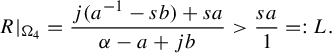 $$ \begin{align*}R|_{\Omega_4}=\frac{j(a^{-1}-sb)+sa}{{\alpha}-a+jb}>\frac{sa}{1}=: L.\end{align*} $$
To compute the contribution of
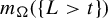 $m_{\Omega }(\{L>t\})$
, we notice that
$m_{\Omega }(\{L>t\})$
, we notice that
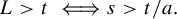 $$ \begin{align*}L>t\iff s>t/a.\end{align*} $$
This is a valid lower bound for s since
 $t/a$
is always positive. The upper bounds on s yield the condition
$t/a$
is always positive. The upper bounds on s yield the condition
 $$ \begin{align*}t/a< (ab)^{-1}\iff b<t^{-1},\end{align*} $$
which yields the integral
 $$ \begin{align*}m_{\Omega}(\{R>t\}\cap \Omega_4)>m_{\Omega}(\{L>t\}) = \int_{b=0} ^{1/t}\int_{{\alpha}=1-b} ^1 \int_{a={\alpha}} ^1 \int_{s=t/a} ^{{1}/{ab}}1\,ds\,da\,d{\alpha} \,db.\end{align*} $$
Evaluating this integral and approximating the result by its Taylor series, we have that
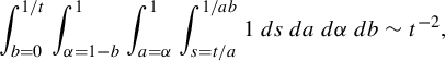 $$ \begin{align*}\int_{b=0} ^{1/t}\int_{{\alpha}=1-b} ^1 \int_{a={\alpha}} ^1 \int_{s=t/a} ^{{1}/{ab}}1\,ds\,da\,d{\alpha} \,db\sim t^{-2},\end{align*} $$
so that a lower bound on the contribution of
 $\Omega _4$
is given by a quadratic function.
$\Omega _4$
is given by a quadratic function.
As a corollary of the measure estimates from above, we obtain that the distribution function for gaps of an affine lattice are supported near 0.
Proof Proof of Theorem 4.4(2)
Note that the volume of
 $\Omega _3$
is given by
$\Omega _3$
is given by
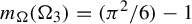 $m_{\Omega }(\Omega _3) = ({\pi ^2}/{6})-1$
. Notice that in the measure estimate of the tail of
$m_{\Omega }(\Omega _3) = ({\pi ^2}/{6})-1$
. Notice that in the measure estimate of the tail of
 $\Omega _3$
in case I, yields that
$\Omega _3$
in case I, yields that
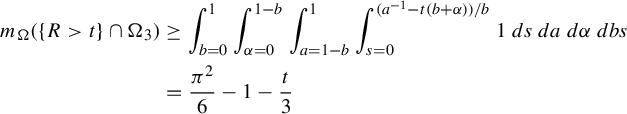 $$ \begin{align*}m_\Omega( \{ R>t \}\cap\Omega_3)&\ge\int_{b=0} ^{1} \int_{{\alpha}=0} ^{1-b}\int_{a=1-b} ^1 \int _{s=0} ^{({a^{-1}-t(b+{\alpha})})/{b}}1\,ds\,da\,d{\alpha} \,dbs\\ &= \frac{\pi^2}{6} -1 - \frac{ t}{3}\end{align*} $$
whenever
 $t<1.$
We only have an inequality because there may be contribution from the other pieces
$t<1.$
We only have an inequality because there may be contribution from the other pieces
 $\Omega _i$
. Hence,
$\Omega _i$
. Hence,
 $$ \begin{align*}\int_0 ^\varepsilon g(t)dt> m_\Omega( \{ R<\varepsilon \}\cap\Omega_3) = \frac{\pi^2}{6}-1 - m_\Omega( \{ R>\varepsilon \}\cap\Omega_3) \ge \varepsilon/3.\end{align*} $$
This contribution is positive for any
 $\varepsilon>0$
and so we conclude that there is support at zero.
$\varepsilon>0$
and so we conclude that there is support at zero.


 Open access