


1. Introduction
It is well known that in turbulent flows over a surface characterised by spanwise heterogeneity, arising because of changes either in surface condition (e.g. roughness or type) or in surface height, secondary flows are created  $via$ the mechanism originally postulated by Prandtl (Reference Prandtl1952). These ‘secondary flows of the second kind’ arise because of spanwise inhomogeneities in the turbulence stresses in the cross-stream plane, which act to produce axial vorticity. There have been numerous studies of such flows, in boundary layers, ducts or open channels. The effects of spanwise changes in surface texture have been investigated by, for example, Chung, Monty & Hutchins (Reference Chung, Monty and Hutchins2018) and Stroh et al. (Reference Stroh, Schäfer, Frohnapfel and Forooghi2020b). In such cases, typified by alternate strips of smooth and rough surface, Hinze (Reference Hinze1967) argued that upwelling occurs over the smooth strips and downwelling over the rough parts, although he recognised that the reverse might be possible, without suggesting conditions when that would occur. He also linked the upwelling regions to those where dissipation of turbulence kinetic energy (TKE) exceeds its production, coinciding with regions of low shear stress. However, this did not ultimately explain the basic source of the axial vorticity patterns; it could be argued that the TKE dissipation/production imbalance is simply the eventual result of the secondary motions produced by the mechanism suggested by Prandtl (Reference Prandtl1952). Anderson et al. (Reference Anderson, Barros, Christenen and Awasth2015) have shown that production of axial vorticity occurs primarily in the regions close to the changes in surface stress.
Such surface stress changes naturally also occur if there are sudden changes in surface height, rather than simply texture (or applied boundary condition) and there have been a number of papers in recent years that discuss the effects of longitudinal ribs of various shapes on channel or boundary layer flows (Hwang & Lee Reference Hwang and Lee2018; Medjnoun, Vanderwel & Ganapathisubramani Reference Medjnoun, Vanderwel and Ganapathisubramani2020; Stroh et al. Reference Stroh, Schäfer, Forooghi and Frohnapfel2020a; Castro et al. Reference Castro, Kim, Stroh and Lim2021; Zhdanov, Jelly & Busse Reference Zhdanov, Jelly and Busse2023). Attention in this paper is concentrated on channel flows containing secondary motions arising because of multiple longitudinal, rectangular ribs of width  $W$ spaced at a distance $S$ from each other, as illustrated generically in figure 1. There have been some similar investigations, largely addressing questions concerning the geometries (in particular, $W/S$ and $H/S$ and the shape of the ribs) which give rise to the strongest and most extensive secondary flow structures and it is generally suggested that the strongest motions occur when $H/S=O{(1)}$, but it is not clear to what extent the precise $H/S$ leading to strongest secondary flows might depend on $W/S$. The papers of Medjnoun et al. (Reference Medjnoun, Vanderwel and Ganapathisubramani2020) and Castro et al. (Reference Castro, Kim, Stroh and Lim2021) provide summaries of the current state of play. The former showed that the secondary flow strength increased roughly linearly with increasing values of a surface heterogeneity parameter, $\xi$, defined as the ratio of the wetted surface area in the gaps between the ribs to that on the ribs themselves. For fixed ratios of rib height to span ( $h/S$), this parameter depends only on $W/S$ and increases with decreasing $W/S$ – i.e. with an increasing width of the relative gap between ribs $(1-W/S)$, consistent with the fact that the secondary motions are likely to increase in strength when there is a larger region in which they can develop between the ribs. However, this conclusion was from a set of rib experiments having a fairly constant $H/S$ (in fact, only varying between 0.8 and 0.88). As the authors pointed out, a more appropriate surface heterogeneity parameter would need to be a function of both $\xi$ and $H/S$. Note that the work of Medjnoun et al. (Reference Medjnoun, Vanderwel and Ganapathisubramani2020) was in the context of boundary layers, so that $H$ was in fact the boundary layer thickness, $\delta$, but there is no reason to doubt that the same arguments hold for the corresponding channel flows. One must be aware, however, that as a boundary layer grows, $\delta /S$ will also grow, so secondary motions may change character as one proceeds downstream, as is evident in the work of Hwang & Lee (Reference Hwang and Lee2018).
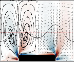
(a) Contours of the axial vorticity superimposed on flow vectors in the spanwise plane for case S12W3 (see table 1). The colour scale runs from deep blue (negative vorticity) to deep red (positive vorticity). In this case, there are three ribs across the span,  $S/W=4$ and $L_y=3.6H$. (b) Sketch of the general computational channel domain for an arbitrary $L_y/S$. Here, $L_z\equiv H=1$ in all cases. In the case shown, $W=2h=0.2H$, $S/W=4$ and the spanwise domain width $L_y$ is $2H$ (much lower than any of the actual cases).

In our earlier work (Castro et al. Reference Castro, Kim, Stroh and Lim2021), we showed how the secondary flow strength varied with  $W/S$, peaking at around $W/S=0.3\unicode{x2013}0.4$, but the cases studied had different values of $H/S$. It was postulated that for a fixed $W/S$, different values of $H/S$ ‘might be expected to change the secondary flow strength’, which is consistent with the proposal by Medjnoun et al. (Reference Medjnoun, Vanderwel and Ganapathisubramani2020) that both $\xi$ and $H/S$ must be important, at least over a certain range of $H/S$. This matter, among others, is addressed in the present work by computing two series of ribbed channel flows having two fixed values of $W/S$ but, in each series, widely varying $H/S$, hence exploring a wider and fuller region of parameter space than previously covered in the literature.
Zampino, Lasagna & Ganapathisubramani (Reference Zampino, Lasagna and Ganapathisubramani2022) have confirmed that both  $(S-W)/H$ and $W/H$ (or, equivalently, both $W/S$ and $H/S$) affect the strength of the secondary motions, by performing comprehensive computations of linearised Reynolds-averaged Navier–Stokes equations, derived by assuming that the rib height (expressed as $h/H$) is a small parameter. They showed that for $W/S=0.5$ and $W/S=0.25$, the peak strength occurs at $H/S\approx 0.7$ and $H/S\approx 0.4$, respectively. It is not clear from that work how large $h/H$ can become before the analysis becomes inappropriate (i.e. before nonlinear effects become significant). However, one of the features of such a linear approach is that the term (in the axial vorticity transport equation) representing convection of the axial vorticity is identically zero. A major motivation of the present work was to assess the behaviour of the different terms in the axial vorticity equation and thus (as it turned out) show that even for $h/H$ as small as 0.025, this convection of axial vorticity remains an important feature of the flow.
The next section outlines the direct numerical simulation (DNS) methodology used and is followed, in § 3.1, by presentation of the basic flow statistics – the mean axial flow and the corresponding turbulence field. Section 3.2 considers the generation of the secondary flows whilst their topology and strength are discussed in §§ 3.3 and 3.4, respectively. The latter section includes comparisons with the linear computations of Zampino et al. (Reference Zampino, Lasagna and Ganapathisubramani2022). Final discussion and conclusions are presented in § 4.
2. Methodologies
All the computations were undertaken using an in-house parallelised, DNS code – CANARD (Compressible Aerodynamics & Aeroacoustics Research coDe) developed at the University of Southampton. The salient features for the present computations were essentially those described by Castro et al. (Reference Castro, Kim, Stroh and Lim2021) and need not be repeated here. Full details of the code are provided by Kim (Reference Kim2007, Reference Kim2010, Reference Kim2013). As indicated by the name, CANARD is a compressible flow solver for which the Mach number ( $M$) should be specified. Here, $M$ was set to 0.25 for all the cases, to keep the compressibility effects minimal and not to cause excessive computational cost. To check that, indeed, the results were only very weakly dependent on $M$, a case (for a plane channel) was run with $M=0.177$ – so that $M^2$ was smaller by a factor of two. The change in, for example, $u_\tau /U_b$ (where $u_{\tau }$ and $U_b$ are the friction and bulk mean velocities, respectively) was negligible and the resulting $u_\tau /U_b$ values from both runs were within 3 % of the result reported by Hoyas & Jiménez (Reference Hoyas and Jiménez2008) at the same Reynolds number and obtained using an incompressible code. This small difference was undoubtedly due to the fact that the latter computed the full channel (height $2H$), unlike the present half-height computations which naturally required a different top boundary condition. Note that the bulk velocity, $U_b$, was defined as the velocity averaged over the channel cross-section area (minus the ribs); the volume flow rate thus varied a little from case to case, depending on the rib size and spacing.
The number of ribs across the span was chosen to ensure that the spanwise domain width,  $L_y$ in figure 1(b), was almost always (at least) ${\rm \pi} H$; $L_y$ depended on the choice of $H/S$ and $W/S$ for each case. In all cases, the axial and vertical domain dimensions were $8H$ and $H$, respectively. All length scales were initially normalised by $H$ in the current DNS, hence $H=1$. A slip wall (symmetry) boundary condition was used on the top wall, periodic conditions at the axial and spanwise boundaries, and no-slip conditions on all bottom and rib surfaces. Distributed over typically 10 368 processor cores, each simulation took around 24 wall-clock hours to reach $t^+_{max}=t_{max}u_\tau /H\approx 62$ during which the flow at the bulk velocity travelled approximately $1000H$. The simulations were largely conducted on the UK national supercomputer ARCHER2, although some initial test runs used the IRIDIS-5 cluster at the University of Southampton.
The axial pressure gradient required to produce a bulk axial velocity ( $Re_b=HU_b/\nu =8950$) was applied at each time step in all cases, designed to yield a channel Kármán number, ${\textit {Re}} _\tau =Hu_\tau /\nu$, of nominally 550, although some runs were undertaken at $Re_\tau \approx 1000$ ( $Re_b=17\,900$) – see table 1 – with appropriately refined grids near the ribs and the bottom wall. This technique led naturally to an axial pressure gradient which fluctuated in time until convergence was achieved, so the latter was checked in each case partly by ensuring that the pressure gradient had stabilised. Actual $Re_\tau$ values for each run are included in table 1, with the final converged $u_\tau$ chosen to ensure that the total shear stress profile collapsed to the expected straight line (see § 3.1). Typically, in the case S8W4 as an example (see table 1), the number of grid points was 1000, 800 and 280 in the axial, spanwise and vertical ( $x,y,z$) directions, respectively, with each rib resolved by 100 and 40 points in the spanwise and vertical directions, respectively. In all cases, the first wall-normal grid spacing was maintained at $\Delta _y^+=\Delta _z^+\approx 1.1$. The same applied to the $h/H=0.05$ and $h/H=0.025$ cases requiring, for the latter cases, 12 vertical cells to resolve the height of the rib. Note that in these cases, the rib sits below the usual log law, since $hu_\tau /\nu \approx 14$.
Details of the various cases computed. Note that all the  $W/S=0.25$ cases are in the left columns and the $W/S=0.5$ cases are in the right columns. Cases having the same $h/H$ and $H/S$ are generally on the same row. The no-rib (i.e. plain channel) case used a domain span of four times the domain half-height. Cases marked with an asterisk are those which did not yield reasonable log law fits in the time- and spatially averaged mean velocity profiles. The four underlined cases were also run at roughly double the Reynolds number, as indicated. Here, $L_y/H$ for each case is the ratio of the bracketed $L_y/S$ value and $H/S$; $d$ (columns 6 and 12) is the zero-plane displacement.

All the results shown herein were obtained using a sufficiently extensive averaging time to ensure convergence. In addition to checking stability of the axial pressure gradient, convergence was assessed by checking that the  $z$-profile of the total time-, spanwise- and axially averaged shear stress collapsed well to the expected straight line. Table 1 lists all the various cases considered here and includes the salient parameter values for each. In summary, two series of computations were undertaken, each with a fixed ratio of rib width to span ( $W/S$), the first having $W/S=0.25$ and the second, $W/S=0.5$, where $S-W$ is the gap between consecutive ribs (recall figure 1 for the geometry). This distinguishes the present work from most earlier studies because, for example, it allowed the strength of the secondary motions to be determined as a function of $H/S$ for fixed $W/S$. In many previous studies, both parameters varied from case to case. The cases listed in table 1 are delineated by nomenclature like S4W1 or S10W25, for example, meaning that the unit span (i.e. a span comprising one rib and the gap between ribs) was $0.4H$ or $1.0H$, with rib widths of $0.1H$ or $0.25H$, respectively. Rib heights were normally 10 % of the channel half-height ( $H$), but additional cases were run with $h/H=0.05$ and 0.025. These latter cases were chosen largely to compare results with the implications of the linearised approach presented by Zampino et al. (Reference Zampino, Lasagna and Ganapathisubramani2022), on the assumption that whilst $h/H=0.1$ would be much too large to expect any such approach to work, $h/H=0.025$ might be small enough to yield usefully comparative results.
3. Results
3.1. Basic statistics – the mean and turbulence flow field
Our emphasis in this paper is on the way in which the secondary flows are generated and how they vary with changes in the surface morphology, specifically  $H/S$ and $W/H$ for fixed $W/S$, but it is appropriate first to illustrate salient features of the mean and turbulence fields. In many cases, we expected the converged, time- and spatially averaged axial mean velocity field, plotted as a function of $z$, to reveal (at least roughly) the usual logarithmic region, expressed as $U^+=({1}/{\kappa })\ln (z-d)^+ + A$, where $d$ is the zero plane displacement, which is the height at which the surface drag appears to act (Jackson Reference Jackson1981) – $d=0$ for a flat wall, of course. A typical mean flow profile is shown in figure 2(a). This case is chosen as it is one giving one of the strongest set of secondary flows for $W/S=0.25$. Castro et al. (Reference Castro, Kim, Stroh and Lim2021) argued that since the bottom boundary on which axial shear is developed is longer than just the unit span (because of the rib surfaces), the effective log-law constants for the specified pressure gradient, $\kappa$ and $A$, must change from the standard values (0.384 and 4.65, respectively) for a plane channel with the same pressure gradient, to values given by
 \begin{equation} \kappa_{rib}=\kappa/\beta \quad\textrm{and}\quad A_{rib}=\beta\left(\frac{1}{\kappa} \ln\beta + A\right)\!, \end{equation}
where  $\beta$ is a function of $W/S$, $h/H$ and $d/h$, given by
 \begin{equation} \beta^2 = \frac{\left(1-\dfrac{h}{H}\dfrac{W}{S}\right) - \dfrac{d}{H}\left(1 - \dfrac{W}{S}\right) }{1+2\dfrac{h}{S} - 2\dfrac{d}{S}}. \end{equation}
In the present ribbed wall cases,  $d$ can be precisely computed from the data using the stress profiles on the bottom wall and the rib's side and top surfaces, as explained by Castro et al. (Reference Castro, Kim, Stroh and Lim2021). For simplicity in the present work, however, it was estimated by, first, adjusting the $u_\tau$ (only nominally set by the applied mass flux) to ensure that the resulting total shear stress profile collapsed to the necessary straight line (as in figure 2b) and then adjusting $d$ to ensure as good a fit as possible between the $U^+$ profile and the expected log law (recognising that, in general, there is no physical reason to expect a good fit). In most cases, this did yield good log law fits and $d$ was found to be usually between $0.4h$ and $0.7h$, a little higher than the average surface height ( $0.25h$ for $W/S=0.25$ and $0.5h$ for $W/S=0.5$). The kink in the velocity profile around $z=h$ is inevitable because the velocity on the rib's top surface is zero, leading to a rapidly falling $U^+$ as $z$ approaches $h$ from above. (Note that below $z=h$, intrinsic averaging was used, i.e. spatial averaging over the fluid region alone.) Profiles at specific spanwise locations do not of course show such kinks nor, indeed, do they generally display a logarithmic region, as demonstrated by Castro et al. (Reference Castro, Kim, Stroh and Lim2021).
(a) Spatially averaged mean velocity profile for case S12W3 ( $H/S=0.833$, $S/W=4$). The dashed line is the standard log-law, with $\kappa =0.384$, $A=4.65$. The solid red line shows the modified log-law (i.e. with the constants given by (3.1a,b)) and the black line shows the data. (b) Spatially averaged shear stresses for S12W3. Reynolds stress, $\overline {u'w'}^+$ (red line), diffusive stress, $\nu \partial \bar {u}^+/ \partial z^+$ (green line), dispersive stress, $\langle \tilde {u}\,\tilde {w}\rangle ^+$ (dashed line) and the sum of all three – the total shear stress (blue line). The straight, red dashed line is the expected total (above the rib).

It is worth emphasising that there is no obvious physical reason why spanwise averaging should necessarily lead to a log law, not least because it has long been known that secondary motions within a boundary layer can lead to distortion of the mean velocity profile (e.g. Mehta & Bradshaw Reference Mehta and Bradshaw1988, and evidenced by the constant  $U$ contours seen in figure 4). The fact that, in many of the present cases, a fit as good as that seen in figure 2(a) occurs must be to some degree fortuitous. There are some cases when, although the total shear stress fits are excellent (which is a necessary measure of good convergence in the computation), the spanwise-averaged velocity profile does not display a satisfactory log law region. This occurred for cases having the higher values of $H/S$, which are indicated in table 1. Note that more of these cases were evident for $W/S=0.5$ than for $W/S=0.25$, consistent with the expectation that the analysis leading to (3.1a,b) is likely to become less satisfactory as $W/S$ increases (see Castro et al. Reference Castro, Kim, Stroh and Lim2021).
Figure 2(b) shows the shear stress profiles for S12W3, corresponding to the velocity profile in figure 2(a). Note that in this case, the dispersive shear stress – a measure of the strength and extent of the secondary flows – is quite large over much of the channel height. It is much larger than the diffusive shear stress which, at this Reynolds number, is always small except in the immediate vicinities of the rib surfaces and  $z=0$, as expected. (For the total stress to continue along the straight line in the region below the rib height, the stress contribution arising from friction on the side walls of the ribs would need to be included. This is an unnecessary nicety for the present purposes.)
The corresponding (normalised) Reynolds normal stresses and dispersive normal stresses are shown in figures 3(a) and 3(b), respectively. In this case, the axial dispersive stress,  $\langle \tilde {u}\,\tilde {u}\rangle ^+$, is of the same order of magnitude as the corresponding Reynolds stress over much of the domain. The other two dispersive stresses ( $\langle \tilde {v}\,\tilde {v}\rangle ^+$ and $\langle \tilde {w}\,\tilde {w}\rangle ^+$) are, however, very much smaller; note they are multiplied by a factor of ten in the figure. At any height, they are no more than approximately 5 % of their corresponding Reynolds stresses. Recall that figure 3(a) shows the Reynolds stresses averaged across the span, ‘hiding’ their spanwise variation. It is the spanwise variations in $\overline {v'v'}$ and $\overline {w'w'}$ (and also $\overline {v'w'}$) which give rise to the secondary motions and the non-zero dispersive stresses, via their spatial, cross-stream gradients. This is explored further in the following sections.
(a) Spatially averaged normal Reynolds stresses for case S12W3 ( $H/S=0.833$, $S/W=4$). (b) Spatially averaged dispersive normal stresses for S12W3. Note that the spanwise and vertical dispersive stresses have been magnified by a factor of ten, making them more visible.

Apart from the distorted constant  $U$ contours (e.g. as in figure 4a), the most obvious visual parameters indicating the presence of secondary flow arising from the inhomogeneous bottom boundary is the non-zero axial vorticity, $\varOmega _x$, and (alternatively) the swirl. Swirling strength is defined as $\lambda _{Ci}\varOmega _x/|\varOmega _x|$, where $\lambda _{Ci}$ is the second invariant of the velocity gradient tensor (Zhou et al. Reference Zhou, Adrian, Balachandar and Kendall1999); this is usually reckoned to be a more satisfactory way of identifying swirling motions. (Vorticity on its own cannot distinguish genuine vortex motions from regions of strong shear.) Figure 4 shows both the vorticity and the swirl, along with cross-stream velocity vectors and cross-plane (quasi-) streamlines, for two cases, S12W3 (figure 4a,c) and S26W13 (figure 4b,d). These cases (one from each series) are chosen as they are close to the $H/S$ values giving the maximal strength of the secondary motions (see § 3.4). In figure 4(a,b), the velocity vectors and streamlines are, for clarity, each shown only on one half of the span. In this and subsequent figures, data shown for the unit span $S$ are obtained by averaging across as many unit spans ( $S$) as there are within the domain width, $L_y$; in the S12W3 case, for example, where $L_y=3.6H=3S$, the three unit span results were averaged. Any slight asymmetry remaining was removed by averaging the data in one half of the span with the corresponding (flipped) data in the other half, so that in all these and similar figures, the data shown on the right half-span are a mirror image of those on the left half-span. (Note that in most cases, the individual span data vary little from span to span across the domain, indicating the generally good symmetry obtained.)
(a,b) Axial vorticity,  $\varOmega _x$, contours for cases (a) S12W3 and (b) S26W13 with cross-stream velocity vectors on the right and (quasi-) streamlines on the left. The solid black lines show the locations where the axial velocity is 90 % of its value ( $U_o$) at the top of the domain which, for a plain channel, would lie along the red dashed lines. (c,d) Corresponding swirl contours for the same two cases. Note the location of the major nodal points (red circles) and saddle points (black squares), including the (half-) saddle at the top centre of the ribs. Note also that in panel (a,b), the arbitrary vorticity colour scale is the same as it is for the swirl colour scale in panel (c,d).

The distortion of the axial velocity field is evident in figure 4(a,b) from the contour lines representing  $U=0.9U_0$, i.e. the line along which the axial velocity is 90 % of its value at the top of the domain ( $U_0$). For a plain channel, this contour would be a straight line at a height of approximately $0.45H$, also shown in the figures. It was distortions such as these which first prompted Prandtl to postulate the existence of what he called ‘secondary flows of the second kind’ (Prandtl Reference Prandtl1952). The topology of the secondary flows illustrated by figure 4 is much as described by Castro et al. (Reference Castro, Kim, Stroh and Lim2021); in the S12W3 case, figure 4(c), there is a saddle point just above the centre of the rib (at approximately $z=2h$), with upward flow above it and downward flow beneath it, and a set of nodal points including two just above the rib and two outboard of it and around $z/S=0.3$. The situation for S26W13, figure 4(d), is very different. Here there is no saddle just above the rib and there is a downward flow all the way from the top boundary to the top of the rib, in contrast with the upward flow that occurs (for S12W3) on $y/S=0.5$ everywhere above the elevated saddle point. The streamline patterns help to clarify this major difference, showing that for S12W3, there is a region of upwelling above the rib, whereas for S26W13, strong upwelling occurs above the rib corners and downwelling above the rib centreline. It is interesting that a similar switch in the secondary flow topology between the two cases seen in figure 4 has also been noted for two cases having fixed $W/S=0.5$ and also fixed $H/S=1$, but with different heights of rough surface (width $W$) with respect to $z=0$ by Stroh et al. (Reference Stroh, Schäfer, Frohnapfel and Forooghi2020b). In that work, when the strip roughness all occurs above the $z=0$ datum, so that there is a significant change in surface elevation at the edge of the strip, the flow looks much like that in figure 4(a), whereas when the roughness largely (but not completely) lies below the $z=0$ datum, there is downwelling above the centre of the roughness strip, as in figure 4(b). However, there is no upwelling at the edges of the strip because these edges are not accompanied by a sharp change in surface elevation as occurs for the case shown in figure 4(b). We discuss in due course the extent to which these structures change with changes in $H/S$ and $W/S$. Meanwhile, it is worth noting that, for rectangular ribs, the linear model by Zampino et al. (Reference Zampino, Lasagna and Ganapathisubramani2022) consistently produced one nodal point directly above each corner (on a vertical line aligned with the side wall) irrespective of $W/S$, which differs from the nonlinear DNS solutions presented here.
It is also of interest that because, as we have seen, the secondary flows often lead to significant distortion of the mean flow, we did not expect any outer layer similarity in the mean flow profiles. Plotting  $(U_o^+-U^+)$ versus $(z-d)/(H-d)$, we found, not surprisingly perhaps, that the divergence from the usual smooth-wall outer flow plot (with $d=0$) at the same Reynolds number was greatest when the secondary flow strength (discussed in § 3.4) was greatest.
3.2. The generation of the secondary flows
These secondary mean flows are uniquely determined by the distribution of the axial vorticity component of the mean flow ( $\varOmega _x=\partial W/\partial y - \partial V/\partial z$), whose steady transport equation can be written as
 \begin{equation} V\frac{\partial\varOmega_x}{\partial y} + W\frac{\partial \varOmega_x}{\partial z} - \nu\left(\frac{\partial^2\varOmega_x}{\partial y^2} + \frac{\partial^2\varOmega_x}{\partial z^2}\right)=S_T, \end{equation}
where  $S_T$ is the source term responsible for production of the longitudinal vorticity. It contains spatial gradients of the Reynolds stresses and is given by
 \begin{equation} S_T = \frac{\partial^2}{\partial y\partial z}(\overline{v'^2}-\overline{w'^2}) + \left(\frac{\partial ^2}{\partial z^2} - \frac{\partial ^2}{\partial y^2}\right)\overline{v'w'} \equiv S_1+S_2. \end{equation}
Note that this form of the transport equation is only valid for a flow that is homogeneous in the axial ( $x$) direction, so that the usual vortex stretching and tilting term is identically zero. For the spanwise homogenous flow in a plain channel, the cross-stream Reynolds stress gradients are also ideally zero so no axial vorticity is produced. Otherwise, as in all the present cases, the two gradient terms $S_1$ and $S_2$ combine to produce $\varOmega _x$, which can then be transported by the first two (convective) terms of (3.3) and diffused by the third, viscous term. The stress gradient terms, $S_1$ and $S_2$, are essentially torques acting on the fluid (Einstein & Li Reference Einstein and Li1958; Nikitin, Popelenskaya & Stroh Reference Nikitin, Popelenskaya and Stroh2021).
As is common with nearly all flows containing external corners (like those in a square duct with no-slip walls, for example), the dominant region of  $\varOmega _x$ production is around the corners themselves, particularly any external (i.e. convex) corners, e.g. Moinuddin, Joubert & Chong (Reference Moinuddin, Joubert and Chong2004) and Hu (Reference Hu2009). Incidentally, even for flows produced using strip roughness (i.e. spanwise heterogeneity produced by alternating strips of low and high surface roughness), where there is no significant change in surface height and thus no external corners, it has been shown that the dominant region of $\varOmega _x$ production occurs in the region very close to the change in roughness (e.g. Anderson et al. Reference Anderson, Barros, Christenen and Awasth2015). Figure 5 emphasises the corner region of the rib in case S12W3, showing contours of vorticity, the source terms $S1$ and $S2$, and their sum $S_T$. Notice first that in regions where they are most dominant (the external corner), the two source terms are of almost equal magnitude but opposite sign, see figure 5(c,d). This ‘butterfly’ pattern, as Khalid, Joubert & Chong (Reference Khalid, Joubert and Chong2004) called it in their experimental study, was noted in the large eddy simulation (LES) study of flow through an annular square duct by Xu & Pollard (Reference Xu and Pollard2001). They found that (in contrast with a concave corner flow) the shear stress (S2) and normal stress (S1) contributions were of nearly equal magnitude. In fact, this feature was evident in a number of the much earlier studies reviewed by Demuren & Rodi (Reference Demuren and Rodi1984) and the pattern is rather like that of sound sources near a corner – dominant production regions of consecutively opposite sign, six of them here but often quadrupoles in the sound source case (Devenport et al. Reference Devenport, Alexander, Glegg and Wang2018). So the resulting total source $S_T$ (figure 5b) arises from the difference of two relatively large terms and is only significant very close to the corner. All three of these terms are very large compared with the diffusive terms, so the convective term closely matches the total source term. The convective term acts to spread significant non-zero vorticity into a much larger region, well away from the dominant source regions near the corner, as figures 5(a) and 4(a) illustrate.
(a) Axial vorticity,  $\varOmega _x$, in the corner region of the ribs in case S12W3. Note that for clarity, the vector lengths are constant, rather than chosen to reflect the values. (b) Total source term, $S_T$, for production of $\varOmega _x$. (c,d) Individual source terms, S1 and S2, respectively. For panels (b)–(d), the colour scale is the same.

We emphasise the behaviour using figures 6 and 7. In these figures, the profiles of the various terms in (3.3) are plotted against  $y'/W$, where $y'$ is chosen so that the unit span covers the range from $-1$ to $+1$. Figure 6 shows spanwise profiles of the three (collected) terms in (3.3) and the vorticity itself, along a spanwise line a little above the top of the rib ( $z=1.3h$). Note first that this close to the rib, the diffusive term is not insignificant in the rib region itself. Second, the total source ( $S_T$) and convective terms are generally dominant and act close to the rib corner locations. Even at this height ( $z=1.3h$), the vorticity has already been spread significantly by the convective term. Figure 7(a) shows similar profiles at $z=2h$ and in figure 7(b), the separate source terms are shown along with the diffusive term. This latter term is clearly insignificant this far above the rib. Notice how closely the two source terms follow each other but with opposite sign. It should also be noted that although the reduction in the maximum value of the total source term ( $S_T$) between the two heights $z=1.3h$ and $z=2h$ is around an order of magnitude, the maximum vorticity reduction is only approximately a factor of three (compare figures 6 and 7a). This emphasises how effective the convective term is in spreading significant axial vorticity into regions where there is practically no generation of vorticity.
Spanwise profiles along  $z=1.3h$ of the axial vorticity (dashed line), and the convective (red line), total source (black line) and diffusive (green line) terms in the vorticity transport equation. The location of the rib is indicated by the black rectangle. Case S12W3.

(a) Spanwise profiles along  $z=2h$ of the axial vorticity (dashed line), and the convective (red line) and total source (black line) terms of the vorticity transport equation. (b) Corresponding profiles for the two separate source terms and the diffusion term (green line). Case S12W3.

Similar behaviour occurs in most of the cases studied. The exceptions are for the cases in which the rib was only  $2.5\,\%$ of the domain height, when diffusional effects are, not surprisingly perhaps, more dominant in the vorticity transport processes close to the rib. This is illustrated in figure 8 for case S20W10 $\_$025, which for clarity shows only the left-hand side of the unit span. At a height near the rib ( $z/h=1.6$), figure 8(a) shows that, in contrast to the S12W3 case in figure 7(a), diffusion roughly balances the total source term and is thus responsible for most of the initial transport of vorticity away from the corner; convection of vorticity is relatively small. (This must also be true for the $h/H=0.1$ cases too, of course, provided one looks close enough to the rib; diffusion is always bound to be dominant close enough to the surface.) Higher up, however ( $z/h=4$, figure 8b), convection again roughly balances the total source term above the rib's corner, but not always elsewhere. Far away from the rib, whatever its height, the diffusion term in the axial vorticity transport equation must always become negligible, so the equation will essentially express a balance between convective transport and the total source term, but the magnitudes of all these will naturally fall as the magnitude of the dispersive stress terms fall; the latter are discussed in § 3.4.
Spanwise profiles along (a)  $z=1.6h$ and (b) $z=4h$ of the axial vorticity (dashed line), and the convective (red line), diffusive (green line) and total source (black line) terms of the vorticity transport equation, for the S20W10 $\_$025 case, having $h/H=0.025$.

If the Reynolds number is sufficiently large, separation must always occur at sharp corners. Given the fine details of the sources of vorticity around the rib corners, it is of interest to ask whether, if the corners were not sharp, these details would be sufficiently different to affect significantly the resulting strength of the secondary flows. This was explored briefly by running the S12W3 case again, but with a rib having rounded corners (with a radius of  $h/4$). Figure 9 shows the comparison, with the rib coloured grey for greater clarity very near to the corner. One obvious effect of rounding the corner is to move the surface separation point from the corner itself (at $y/S=0.375$, figure 9a) to a little way inboard ( $y/S\approx 0.43$, figure 9b), as evident from the sign of the velocity vectors just above the surface. Although the details of the various contributions to (3.3) differ somewhat, figure 9 indicates that the overall strength of the resulting vorticity is not hugely changed by rounding the rib corner (but see later), although it is noticeably weaker. With a rounded corner, the nodal point above the rib (at $y/S=0.45$, $z/S=0.125$) for the sharp corner case has moved a little lower and nearer to the rib centreline and, in addition, the centreline saddle has moved down from above $z/S=0.15$ to approximately $z/S=0.125$. These are only minor changes in critical point locations and the topological structure of the secondary flow is not changed at all. We conclude that corner rounding does not lead to large changes in the overall secondary flow field unless, presumably, the change is much more severe than used here (e.g. from a rectangular to a semi-circular rib). It is the large-scale surface features which determine the overall topology, rather than their fine details.
Axial vorticity and cross-stream velocity vectors in the corner region (a) without and (b) with a rounded corner, for case S12W3. The (arbitrary) vorticity scale is the same in both figures. Note the saddle of separation at approximately  $y/S=0.43$ and the centreline saddle at $z/S=0.13$, shown by black squares in panel (b), and the nodal points (red circles) in panel (a,b).

3.3. The topology of the secondary flows
It was noted earlier that the vertical flow direction above the rib centre depends on the controlling parameters,  $H/S$ and $W/S$ (compare figures 4a and 4b). The different locations of the salient critical points (nodes and saddles) reflect the changes in these parameters and they are driven essentially by the available space for development of the large recirculating regions above the rib. In all of the $W/S=0.25$ cases, there is a saddle point above the rib centre, as seen in figure 4(a,c), but this saddle gradually moves upwards as $H/S$ decreases. Figure 10(a,b) show the two extreme cases for $W/S=0.25$. For $H/S=2.5$ (S4W1, figure 10a), the saddle point above the rib centreline is around $z_s/h=1.3$, whereas by $H/S=0.385$ (S25W65, figure 10b), it has moved up relative to the rib height to $z_s/h=4.2$.
Vorticity, (quasi-) streamlines and cross-stream vectors in the extreme cases for (a,b)  $W/S=0.25$ and for (c,d) $W/S=0.5$. (a) $H/S=2.5$, case S4W1; (b) $H/S=0.385$, case S25W65; (c) $H/S=2.5$, case S4W2; (d) $H/S=0.25$, case S40W20. Red circles are nodes, black rectangles are saddles. The vorticity scales are arbitrary and the same for all plots, and the vectors’ scale is the same in each. The solid black lines are the $U=0.9U_0$ contours. Note the much smaller domain depths in panel (b,d), as is clear from the axis scales.

It is emphasised that we have not included all the critical points in these figures. In particular, we exclude those in regions where the cross-stream velocities are particularly small compared with those delineating the main secondary motions, so that exact streamline paths are more uncertain. The complete topology within typical domains is explained more fully by Castro et al. (Reference Castro, Kim, Stroh and Lim2021). For the  $W/S=0.5$ cases, there are situations where the central saddle above the rib disappears, so that flow moves downwards from the top half-saddle all the way to the rib surface, as seen in figure 4(d) for S40W20 ( $H/S=0.25$). Figure 10(c,d) show the two extreme cases for $W/S=0.5$. The only case in figure 10 which does not have a region of upward flow above a free saddle above the rib is that of $W/S=0.5$, $H/S=0.25$ – figure 10(d). However, for $W/S=0.5$, all those cases with $H/S\le 0.714$ have downward flow all the way from the top of the domain to the rib surface. In every case, half-saddles at $y/S=0.5$ exist on the rib surface and the top of the domain and, although they are not included in the figures, there are also always saddles of separation at the rib corners (except when the corner is rounded, as explained in § 3.2). Note also that in the two $H/S=2.5$ cases shown in figure 10, there is very little distortion of the axial velocity field, even though the overall strength of the secondary flow is somewhat larger than it is for the other two cases (see § 3.4). This is because in the former cases, all the important secondary flows occur in a vertically small region of the total domain depth, whereas for S25W65 (figure 10b) and S40W20 (figure 10d), the domain depths are themselves relatively small (compared with the span) so that the secondary flows have a strong influence over the entire domain. The weakness of the secondary flows above approximately $z/S=1$ in the $H/S=2.5$ cases is evidenced not least by the very short vectors over most of the height of the domain – they are in fact hardly discernible compared with those at lower heights (below approximately $z/S=1$ in figure 10a,d).
In general, of course, the existence and location of any saddle point above the rib centreline must depend on the three independent geometrical parameters:  $W/S, H/S$ and $h/H$ (as well as the Reynolds number). The movement of this saddle as $H/S$ varies but with fixed $W/S$ and $h/H$ is illustrated by figure 11. In the $W/S=0.5$ cases, once $H/S$ exceeds approximately 0.7, it is clear that a saddle appears above the rib at approximately $z_s/h=6$ and then gradually moves downward until the situation shown in figure 10(c) for case S4W2 ( $H/S=2.5$). However, when $W/S=0.25$ there is always such a saddle point above the rib, again moving down as $H/S$ increases from 0.385 to 2.5 – the two extreme cases shown in figure 10(a,b). This difference is evident also in the results of Wang & Cheng (Reference Wang and Cheng2006), who studied open channel flow over ribbed (and striped) surfaces: they showed that in the rib cases, for $H/S=0.53$, there was no upper saddle point when $W/S=0.5$, but one appeared (around $z/h=6$) when $W/S=0.33$. In the present cases, most of the saddle point movement occurs before $H/S$ reaches approximately unity, particularly for the much smaller rib ( $h/H=0.025$) – see the red symbols in figure 11(b). Plotting the above-rib saddle location as a function of $H/W$, as done in figure 11(c), suggests that it may be this parameter, almost independently of $W/S$, that controls when the topology changes, with the saddle moving down from the top boundary once $H/W$ exceeds around 1.3. We confirmed that by running three additional cases for $W/S=0.25$ (which are not included in table 1), having $H/W=1.25$, 1.33 and 1.43; the resulting saddle point locations are included in figure 11(a,c) and identified as solid red triangles.
Movement of the above rib saddle point as  $H/S$ varies. The dashed lines indicate the top of the domain. Triangles refer to $W/S=0.25, h/H=0.1$, circles to $W/S=0.5, h/H=0.1$ and red circles in panel (b) are for $W/S=0.5, h/H=0.025$. Red triangles in panel (a,c) refer to the three extra $W/S=0.25, h/H=0.1$ cases (not listed in table 1).

Various other nodes and saddles (not shown) appear well away from the rib and at differing locations as  $H/S$ varies, particularly for large $H/S$ but, as noted above, these occur in places where the cross-stream velocity magnitudes are very low compared with those nearer to the rib and there is little to be gained by exploring them in detail. It is more important to explore the overall strength of the secondary flows and we discuss this next.
3.4. The strength of the secondary flows
3.4.1. Initial remarks
Recall from § 3.1 and figure 3 that the axial dispersive stress can be of similar magnitude to the axial normal stress, whilst the other two normal dispersive stresses are relatively very small indeed (but enough to generate the secondary flows, as explored below). It is expected that the magnitude of the axial dispersive stress will depend on the strength of the secondary flows. Before discussing the latter, we show in figure 12(a) profiles of  $\langle \tilde {u}\,\tilde {u}\rangle ^+$ for the various cases with $W/S=0.25$ and, in figure 12(c), similar profiles for $W/S=0.5$. In figure 12(b), $\langle \tilde {u}\,\tilde {u}\rangle ^+$ at fixed $z/h$ (in the outer region of the channel) is shown as a function of $W/H$. It is evident that $\langle \tilde {u}\,\tilde {u}\rangle ^+$ can be large across the whole domain, emphasising earlier conclusions in the extant literature (e.g. Zampiron, Cameron & Nikora Reference Zampiron, Cameron and Nikora2020) and the evidence of figure 10(b,d), which indicate very significant distortion of the axial velocity field (as evidenced by the $U=0.9U_o$ contour). Peak magnitudes occur when $W/H$ is approximately 0.4 ( $H/S=0.625$) in the $W/S=0.25$ cases and approximately 1.6 ( $H/S=0.313$) in the $W/S=0.5$ cases. When $H/S$ is large (2.5, say), the dispersive stress is only significant for $z/H\le 0.2$, suggesting that the secondary motions must be very weak in the outer part of the channel and thus have little influence on the axial velocity field, just as implied by figure 10(a,c), which show that the $U=0.9U_o$ contour is virtually flat when $H/S=2.5$.
(a,c) Profiles of  $\langle \tilde {u}\,\tilde {u}\rangle ^+$ for $W/S=0.25$ and 0.5, respectively (above $z=h$). The legends give values of $W/H, H/S$. (b) Profiles of $\langle \tilde {u}\,\tilde {u}\rangle ^+$ at fixed heights of $z/h=0.6$, 0.7 and 0.8 for the two series. $S/W=0.25$ data are red triangles; $S/W=0.5$ data are black circles.

There are various ways in which one could assess the secondary flow strength more directly. A particularly useful approach is to determine the total integrated kinetic energy per unit area in the cross-stream mean motions, which we call KE $^+$, as defined by
 \begin{equation} \text{KE}^+=\int_0^{1}\int_0^1\frac{1}{2u_\tau^2}(V^2+W^2)d(y/S)d(z/H). \end{equation}
 Before considering how this quantity varies with  $H/S$ or $W/H$ and with rib height, $h/H$, and given that it is normalised using the friction velocity, $u_\tau$, it is pertinent to ask how $u_\tau$ varies with rib height. Figure 13 shows the variations of both $u_\tau /U_b$ and $U_0^+$ (the mean axial velocity at $z=H$) with $h/H$ for the S16W4 cases. ( $U_b$ is the bulk velocity which, it will be recalled, was exactly the same in all cases.) It is evident that the changes in $u_\tau$ are quite small. As expected, an increase in rib height from zero (the plain channel) increases the axial pressure gradient (and thus the $u_\tau$) needed to maintain the same mass flux; $U_0^+$ consequently decreases somewhat. At fixed $h/H$, there is a monotonic fall in $u_\tau /U_b$ as $H/S$ falls (unlike the changes in KE $^+$ with falling $H/S$), simply because $U_b$ was fixed (see § 2) whilst the contribution of the rib to the bottom surface area falls; there is thus no direct link between secondary flow strength and the drag. (Note, however, that if $W/H$ and $H/S$ are both fixed, changes in $h/H$ lead to concomitant changes in secondary flow strength and drag, as implied by figures 13 and 14(b), and as shown by Stroh et al. (Reference Stroh, Schäfer, Forooghi and Frohnapfel2020a).)
Variation of (a) friction velocity  $u_\tau /U_b$ and (b) $U_0^+$ with rib height, for the S16W4 case ( $H/S=0.625$, $W/S=0.25$). Note the false origins for the vertical axes.

Total cross-stream kinetic energy, KE $^+$ as (a) $H/S$ and (b) $W/H$ vary. The legends identify the two main sets of data. In panel (a), the single solid green triangle is case S12W3 but with a rounded corner, the two red plusses and the two orange crosses refer to the ${\textit {Re}}=1000$ cases for $W/S=0.25$ and $W/S=0.5$, respectively. In panel (b), the red dotted line (with small red circles) shows data for $W/S=0.5$ with the small rib ( $h/H=0.025$) and the vertical red lines join data for ribs of height $h/H=0.05$ and $h/H=0.025$ to the main sequences. The (long-)dashed red line is from the linearised model of Zampino et al. (Reference Zampino, Lasagna and Ganapathisubramani2022) (with $h/H=0.025$) and the horizontal red dotted line is for a plain channel (see text).

Figure 14 shows how KE $^+$ varies with $H/S$ or $W/H$. The figures change very little in shape if the kinetic energy is normalised by the integrated kinetic energy per unit area of the mean axial velocity, which we could call UKE $^+$, because the latter typically varies within only ${\pm }10\,\%$ of the average of approximately 138 over all the ( $h/H=0.1$) cases. Incidentally, this latter value, compared with the typical KE $^+$ values in figure 14, emphasises how weak the secondary motions are: their ratio (KE/UKE) hardly ever exceeds $10^{-4}$ across all the cases. We emphasise too that using total area-integrated swirl as an alternative to KE $^+$ yields results very similar to those in figure 14. Furthermore, if KE $^+$ is measured only over the top 70 % of the domain (thus ignoring contributions closer to the ribs), the results are again very similar to the latter; the locations of the peak values hardly change. The general behaviour of KE $^+$ versus $W/H$ is very similar to that of the axial dispersive stress shown in figure 12(b), as would be expected. It is notable, however, that for both series, the peak KE $^+$ occurs at slightly smaller $W/H$ values than those that yield the (local) peak dispersive stresses (cf. figures 14b and 12b); the difference is not large and varies somewhat depending on which height is chosen for the latter. By comparison between figures 11(a) and 14(a), it is interesting to note that although, for $W/S=0.5$, there are large and non-monotonic changes in KE $^+$ as $H/S$ varies up to approximately 0.7, the upper saddle point remains fixed at the upper boundary, only beginning to sink towards the rib when KE $^+$ is well beyond its peak. It is also notable that for $H/S\ge 1$, the cases having a stronger KE $^+$ (i.e. for $W/S=0.25$) lead to a saddle point closer to the rib, which is perhaps not surprising.
Figure 14(b) includes data for the  $h/H=0.025$ cases. As $h/H\to 0$, the geometry naturally becomes that of the regular plain channel. Because of the limited spanwise extent of our plain channel DNS, we do not expect the secondary flows to be entirely absent (see Lozano-Durán & Jiménez Reference Lozano-Durán and Jiménez2014, for a discussion of domain size effects). Figure 14(b) includes the KE $^+$ value (0.00082) for the plain channel with a span of $4H$. This is a factor of $4.5\times 10^{-6}$ times the integrated axial kinetic energy (UKE $^+$) and one might expect it to fall further with increasing spanwise domain width. It is possible that the data for the $h/H=0.025$ cases, particularly, might be affected by the finite domain width. We do not believe, however, that such effects are very significant, not least because the minimum KE $^+$ values in these cases are approximately twice the plain channel value, but also because the location of the secondary motions is clearly fixed in each case by the rib geometry. Before exploring (in § 3.4.5) the conditions which lead to peak energies in the secondary flows, there are three issues in relation to figure 14 that are worth some discussion.
3.4.2. Reynolds number
Consider first the effect of changes in Reynolds number. Recall that four cases (S8W2 and S16W4 for  $W/S=0.25$, and S8W4 and S26W13 for $W/S=0.5$) were run at roughly double the Reynolds number ( ${\textit {Re}}_\tau =Hu_{\tau }/\nu \approx 1000$), see table 1. The resulting KE $^+$ data are included in figure 14(a). It is evident that for the two larger $H/S=1.25$ cases, remote from the $H/S$ values which give maximum peak energy, doubling ${\textit {Re}}_\tau$ makes an insignificant change in the total cross-stream kinetic energy. For the two cases representing situations for which KE $^+$ is near its peak (S8W4, $H/S=0.385$ for $W/S=0.5$, and S8W2, $H/S=0.625$ for $W/S=0.25$), KE $^+$ falls noticeably with increasing Re $_\tau$ but only in the S8W4 case. Visualising the cross-stream contours of the vorticity or swirl shows that in the case where there is a larger gap between ribs ( $W/S=0.25$), allowing more room for the motions to develop and expand in the gap, the vortices in the gap become significantly ‘tighter’ as ${\textit {Re}}_\tau$ increases; they therefore spread rather less into the region above the rib and in the gap, but this has little overall effect on the area-averaged KE $^+$. However, the tightening of the vortices with increased ${\textit {Re}}_\tau$ in the S8W4 case seems even more noticeable and this significantly reduces their area so that the area-averaged KE $^+$ (i.e. averaged over the entire domain) reduces. This general ‘tightening’ of the vortices as ${\textit {Re}}_\tau$ increases is not surprising and was noted in our earlier work (Castro et al. Reference Castro, Kim, Stroh and Lim2021). Overall, increasing ${\textit {Re}}_\tau$, even by the factor of two used here, has only weak effects and does not alter the topology of the secondary flows, as found by previous authors (e.g. Vanderwel & Ganapathisubramani Reference Vanderwel and Ganapathisubramani2015).
3.4.3. Corner effects
Consider secondly the effect of rounding the rib corners. It was noted in § 3.2 that this leads to a small weakening of the vorticity around the corner (compare figures 9a and 9b). However, figure 14(a) shows that the overall KE $^+$ is increased a little by corner rounding. This is because the major two outboard vortices centred at approximately $z/S=0.3$, see figure 4(c), actually strengthen somewhat with a rounded corner, despite the vorticity immediately near the corner becoming weaker and despite also the fact that the source and convective terms in the axial vorticity transport equation have a very similar structure and strength. However, the secondary flow is directed smoothly around the corner, gaining strength as it goes and sweeping upwards at the centreline with greater velocity than if the flow were forced to separate by a sharp corner. This, again, is perhaps not surprising and it is consistent with the findings of Medjnoun et al. (Reference Medjnoun, Vanderwel and Ganapathisubramani2020), in that obstacle shapes that promote merging of the flow being deflected (like a triangular rib, for example) generate a stronger central upwash. Such shapes, like our rounded corner rib, create less of an extreme resistance to the spanwise flows below $z=h$, with concomitant increase in strength of the secondary flows, as also noted in other studies (see Goldstein & Tuan Reference Goldstein and Tuan1998; Hwang & Lee Reference Hwang and Lee2018, for example). Again, however, the overall effect is not extreme – a mere 16 % increase in KE $^+$ on rounding the rib corners in this particular case. We speculate that the effect is likely to be smaller for $H/S$ values away from those leading to peak secondary flow energy.
3.4.4. Comparisons with the linear model
Figure 14(b) plots the same data against  $W/H$, because this more easily allows comparison with the implications of the linearised model of Zampino et al. (Reference Zampino, Lasagna and Ganapathisubramani2022). The latter is not expected to be satisfactory for a rib as large as $h/H=0.1$, but the figure includes our $h/H=0.025$ data for $W/S=0.5$ along with the implications of the model of Zampino et al. (Reference Zampino, Lasagna and Ganapathisubramani2022) for that size rib. It is interesting that the model predicts the overall strength of the secondary motions reasonably well, but the peak occurs at a rather smaller $W/H$ (around 0.6, compared with 0.8 from our DNS). With the rib four times as large, the peak in our DNS data occurs at even larger $W/H$ (approximately 1.3), but its magnitude is far lower than would be implied by the linear model of Zampino et al. (Reference Zampino, Lasagna and Ganapathisubramani2022). With $h/H=0.1$ (not shown), this yields very much larger KE $^+$. The peak naturally occurs at the same $W/H$ but its value is in excess of 0.052. This is 16 times larger than with $h=0.025H$, since the rib is four times larger and the model is linear, so that secondary velocities are four times larger.
It seems clear that for any but the smallest ribs, the linearised model does not capture the secondary motions adequately, no doubt partly because it cannot capture the precise details of the relative size of the terms in the axial vorticity transport equation. This must surely be true whatever the shape of the ribs. In particular, the convective terms in the linearised version of (3.3) are completely absent from the model because they are second order in the perturbation velocities. This means that the production of axial vorticity by the source terms has to be exactly balanced by diffusion everywhere. It was shown in § 3.2 that only for the small rib height cases and close to the rib is the flow characterised by a balance between the source and diffusion terms, with convection being relatively very small, see figure 8(a) for  $z/h=1.6$. Larger ribs inevitably have convection balancing production almost everywhere (see figure 6 for $z=1.3h$), so that the linearised model inherently cannot capture the flow processes. Perhaps the crucial point regarding the linear model is that it assumes the rib height is small compared with any inner (as well as outer) scale, which requires $hu_\tau /\nu \ll 1$. The present computations with $h/H=0.025$ have $hu_\tau /\nu \approx 12$, which hardly fulfils that requirement. Even for the present Reynolds numbers ( $Hu_\tau /\nu \approx 550$), one would need a rib at least an order of magnitude smaller, but such a rib size is likely much smaller than in typical engineering or environmental applications of these flows, unless one is adding ribs (‘riblets’ in the usual terminology) to reduce the surface drag, but in that case, they would be much closer together. The recent work of von Deyn, Gatti & Frohnnapfel (Reference von Deyn, Gatti and Frohnnapfel2022) confirms that riblets cease to yield drag reductions, giving increased drag instead (undoubtedly linked to the development of secondary flows), once the viscous-scaled square root of the groove area between ribs exceeds approximately 17 (see also García-Mayoral & Jiménez Reference García-Mayoral and Jiménez2011; Modesti et al. Reference Modesti, Endrikat, Hutchins and Chung2021). In terms of the present parameters, this scaled groove area can be written as
 \begin{equation} l_g^+= \sqrt{(S/H-W/H)h/H}{\textit{Re}}_\tau. \end{equation}
Our  $h/H=0.025$, $W/S=0.5$ cases have $55 \le l_g^+ \le 94$. Reducing the rib height by an order of magnitude would, at the lower end of this range, yield $l_g^+ \ge 17$ (and $h^+\ge 1.3$) which is perhaps marginal for the linear analysis to be appropriate (although higher Reynolds number might widen the $h/H$ range yielding secondary flows whilst still expecting the linear analysis to be appropriate). It would be a mistake to conclude that any smaller rib height in our cases would be likely to yield drag reduction (and no secondary flows), since the ribs are much too far apart for the usual drag reduction mechanisms to operate. As shown by von Deyn et al. (Reference von Deyn, Gatti and Frohnnapfel2022), for example, these require $S$ and $h$ to be of the same order. Simply reducing $h$ in the present cases leads to a surface morphology more like a flat surface with occasional very small excrescences.
A further indication of the expected tendency for the linear model to work better as  $h/H\to 0$ is seen in comparing the streamline patterns for a typical case. Figure 15 shows a repeat of (the left-hand side of) figure 4(b) ( $h/H=0.1$) along with the corresponding flow for $h/H=0.025$. The overall topology is the same, but the main central vortex above the rib in the former case is significantly narrower when $h/H$ is only 0.025. It seems likely that for an even smaller $h/H$, this central vortex would narrow further. The linear model does not produce such a vortex at all, showing again that even for a rib whose height is only 2.5 % of the domain height, there are flow features which cannot be captured by that model. Note that, as discussed by von Deyn et al. (Reference von Deyn, Gatti and Frohnnapfel2022), for genuine riblets where both $S^+$ and $h^+$ are of the same order (or, in the case of $h^+$, much less) than the viscous sublayer height, there are linear models which compute the small-scale flows around the riblets themselves and can capture the changes in drag quite successfully, although they do not address the issue of the large-scale secondary flows discussed in this paper (see for example Bechert & Bartenwerfer Reference Bechert and Bartenwerfer1989; Luchini, Manzo & Pozzi Reference Luchini, Manzo and Pozzi1991).
Streamline patterns and  $x$-vorticity for S26W13 ( $H/S=0.385$), with (a) $h/H=0.1$ and (b) $h/H=0.025$. The (arbitrary) colour scale is the same for both cases.

3.4.5. Geometries for maximal secondary flow strength
Finally, we consider the geometrical conditions for the most energetic secondary motions. The data of both Castro et al. (Reference Castro, Kim, Stroh and Lim2021) and Vanderwel & Ganapathisubramani (Reference Vanderwel and Ganapathisubramani2015) suggest that the maximum secondary flow strength occurs when  $W/S$ is approximately 0.4 but, as noted earlier, this must depend significantly on specific values of $H/S$. The $W/S=0.5$ data from the present computations – not very far from $W/S=0.4$ – show that the peak energy is actually lower than it is for the $W/S=0.25$ cases (see figure 14) but, for both sets, the strength is indeed very dependent on $H/S$ (or, equivalently, $W/H$). It is clear from figure 14(a) that the peak energy occurs around $H/S=0.8$ in the $W/S=0.25$ cases, whereas for the $W/S=0.5$ cases the peak occurs around $H/S=0.4$. These correspond to $W/H=0.3$ and $W/H=1.3$, respectively.
By studying boundary layer flow over ribs of various different shapes (but roughly the same  $h/H$ and $S/H$, where $H$ is the boundary layer thickness), Medjnoun et al. (Reference Medjnoun, Vanderwel and Ganapathisubramani2020) argued convincingly that the influence of the surface heterogeneity on the flow must be a function not just of $H/S$, as previous work indicates, but also of a surface parameter, $\xi$, defined as the ratio of the perimeters of the elevated and recessed areas. So they suggested that a surface heterogeneity parameter $\mathcal {H}$ could be written as $\mathcal {H}=F(\xi,{S}/{H})$. In the case of rectangular ribs, $\xi$ is given by
 \begin{equation} \xi = \frac{S-W+2\bar{h}}{W+2(h-\bar{h})}, \end{equation}
where  $\bar {h}=h({W}/{S})$ is the average surface height. Following the suggestion of Medjnoun et al. (Reference Medjnoun, Vanderwel and Ganapathisubramani2020) that $\mathcal {H}=F(\xi,{S}/{H})$, one could postulate a heterogeneity parameter like, for example, $\mathcal {H}=\xi (S/H)^n$. Figure 16(a) shows the KE $^+$ data as a function of $\mathcal {H}$, with $n$ chosen as $n=1.3$ to yield a reasonable collapse in the location of the peak KE $^+$ for the two main series having $h/H=0.1$. In that respect, $\mathcal {H}$ works well. However, the $h/H=0.025$ series (having $W/S=0.5$) has a peak KE $^+$ at a very different location, suggesting that $\mathcal {H}$ is not sufficient for predicting when the peak KE $^+$ occurs. This is in fact self-evident, for if $W/S=0.5$, the parameter $\xi$ is always unity independently of $h/H$ for a given $H/S$. It would be possible to add a further functional dependence to the heterogeneity parameter – $\mathcal {H}=(\xi, {S}/{H}, h^+)$ for example – but it is not obvious what precise dependence would be appropriate, nor what physical argument might be offered to explain it.
(a) Total cross-stream kinetic energy, KE $^+$, as a function of $\mathcal {H}=\xi ({S}/{H})^n$ with $n=1.3$; (b) KE $^+$ factored by KE $^+_{ref}$ (with $\sigma _0 = 0.1$ and $k=0.25$); (c) with $\mathcal {H}=\xi ({S}/{H})^n$ factored by $h^{+2k}$.

Note also in figure 16(a) that the magnitudes of KE $^+$ do not collapse. Using a scaling argument applied to the axial vorticity transport equation (see Appendix A), it is possible to argue that a representative kinetic energy (KE $^+_{ref}$) can be written as
 \begin{equation} \text{KE}^+_{ref} = \frac{1}{2}(W^{+2}_{ref}+V^{+2}_{ref})\approx\frac{\sigma^2(S-W)^2+h^2}{2HS}, \end{equation}
where  $\sigma$ is an arbitrary parameter ( $\sigma <1$). This representative KE $^+_{ref}$ can be used to scale the KE $^+$ shown in figure 16(a) and the resulting scaled values are shown in figure 16(b). Note however that since the horizontal length scale $\Delta y=\sigma (S-W)$, used in the derivation of KE $^+_{ref}$, should likely depend on $h^+$ (since as $h^+ \to 0$, the length scale must also tend to zero), we have written the $\sigma$ in (3.8) as $\sigma =\sigma _0 h^{+k}$. In all the present cases, with $\sigma _0=0.1$ and $k=0.25$, this yields horizontal scales between approximately 0.2 and 0.3 of $S-W$, which seems entirely reasonable. The data in figure 16(b) for $h/H=0.1$ suggest that the resulting $\text {KE}^+/\text {KE}^+_{ref}$ yields a fair collapse. Again, however, the peak scaled KE $^+$ remains horizontally mismatched for the $h/H=0.025$ cases, emphasising the importance of $h/H$ or $h^+$, beyond that included in (3.8), in setting the strength of the secondary motions. Scaling $\mathcal {H}=F(\xi,{S}/{H})$ by an additional factor of $h^{+2k}$ can (as hypothesised earlier), with an appropriate value for the index $k$, lead to a reasonable collapse of all three series, as shown in figure 16(c) but, again, it is not obvious whether such scaling would work more generally. Further study for additional $W/S$ values would be necessary to determine this.
4. Final discussion and concluding remarks
An unsurprising conclusion of the present work is the confirmation that in the case of a channel containing longitudinal rectangular ribs, generation of axial vorticity arises predominantly very close to the corners of the ribs – i.e. the locations of a sudden change in surface stress – where there is the greatest inhomogeneity in the cross-stream Reynolds stresses. It is largely convection of that axial vorticity that is the main means of distributing the vorticity across the channel. This agrees with the conclusion of Anderson et al. (Reference Anderson, Barros, Christenen and Awasth2015), who used LES to study cases in which the spanwise heterogeneity was formed by alternating axial strips of high and low roughness, with (in the present terms) fixed values of  $W/S\approx 0.18$ and $H/S\approx 0.32$ (i.e. $1/{\rm \pi}$). Axial vorticity generation close to the edges of the roughness strips was essentially independent of the ratio of the two roughness ‘strengths’. Our results show that the general behaviour is also independent of $W/S$, $H/S$ and $h/H$. It is worth noting that secondary flows similar to those discussed here can also occur above three-dimensional rough surfaces, as illustrated by Kaminaris et al. (Reference Kaminaris, Balaras, Schulz and Volino2023), who studied the evolution of a turbulent boundary layer over various configurations of truncated cones. However, in that case, there was a significant influence of the vortex stretching/tilting term (VST) in the axial vorticity transport equation, particularly near the leading edge of the roughness, and the authors argued that the resulting secondary flows were thus essentially of Prandtl's first kind. Although they had some similar features, they should therefore not be confused with the secondary flows studied here, which arise in the complete absence of the VST, because of the axial homogeneity of the surface topology.
A further conclusion is that very close to the rib surfaces, diffusion will always be significant but, at least for the largest ribs studied here ( $h/H=0.1$), it hardly contributes to the dispersion of the vorticity, which is largely controlled by convection. This remains true for the smallest ribs ( $h/H=0.025$, $h^+\approx 12$). A direct implication, constituting another of our main conclusions, is that models based on linearised equations cannot generally reproduce either the maximum strength of the secondary motions, or where that occurs as a function of $W/H$, because such models implicitly do not include the convective terms in the axial vorticity equation (since they are second order). It was argued that reducing the rib size sufficiently to satisfy the linear model assumption that the rib scale must be smaller than the inner length scale of the flow would (at least for ${\textit {Re}}_\tau \sim 500$) lead to ribs so small that they merely become occasional excrescences on an otherwise flat surface. At sufficiently high Reynolds number, however, there maybe a range of $h/H$ within which drag is increased and a linear model is appropriate. This is perhaps worth further study. Additionally, we found in the present cases that the effects of rounding the rib corners or doubling the Reynolds number are small.
Finally, we conclude also that for a fixed rib height ( $h/H=0.1$), the peak secondary flow strength occurs when the surface heterogeneity parameter introduced by Medjnoun et al. (Reference Medjnoun, Vanderwel and Ganapathisubramani2020), (3.7), but modified by an appropriate power of $S/H$ – i.e. $\mathcal {H}=\xi ({S}/{H})^{1.3}$ – has a value around three, independent of $W/S$. However, this seems not to carry over to other values of $h/H$, not surprisingly, and it is not clear how a more general parameter should be formulated, although it has been shown that using an additional factor of $h^+$ to scale both the surface heterogeneity parameter $\mathcal {H}=\xi ({S}/{H})^{1.3}$ and the area-integrated secondary flow kinetic energy can lead to a reasonable collapse of all the data.
Acknowledgements
The authors would like to thank Drs Lasagna and Zampino and also Professor Ganapathisubramani for access to their data and for very helpful discussions, particularly regarding their linear model. They also thank the reviewers, who provided a number of helpful suggestions.
Funding
The support of the EPSRC for the computational time made available on the UK supercomputer ARCHER2 by the UK Turbulence Consortium (EPSRC EP/X035484/1) is gratefully acknowledged.
Declaration of interests
The authors report no conflict of interest.
Data access statement
All data supporting this study are available from the University of Southampton repository at https://doi.org/10.5258/SOTON/D3034.
Appendix A. Determining a representative cross-stream kinetic energy
The axial vorticity transport equation (3.3) can be written in terms of the secondary velocities (since  $\varOmega _x = \partial W/\partial y - \partial V/\partial z$) as
 \begin{align} V\left( \frac{\partial^2W}{\partial y^2} - \frac{\partial^2V}{\partial y\partial z}\right) +W\left( \frac{\partial^2W}{\partial z\partial y} - \frac{\partial^2V}{\partial z^2}\right) - \nu\left(\frac{\partial^3W}{\partial y^3} - \frac{\partial^3V}{\partial y^2\partial z} +\frac{\partial^3W}{\partial y\partial z^2}-\frac{\partial^3V}{\partial z^3}\right)=S_T. \end{align}
Here, we consider a small area between two successive ribs where a good level of secondary flow is developed (as shown in figure 5) but is not too close to the ribs where the source term is particularly significant. We may define the size of the ‘reference’ area with  $\Delta z=h$ and $\Delta y=\sigma (S_r-W_r)$, which is a fraction of the gap between successive ribs determined by the arbitrary parameter $\sigma < 1$. It is suggested in § 3.4.5 that this parameter may have a form of $\sigma =\sigma _0 h^{+k}$, where $\sigma _0$ and $k$ are constants. Here, $W_r$ and $S_r$ are used to distinguish them from the cross-stream velocity $W$ and the source term $S_T$. In this reference area, we evaluate the scale of each term of the equation. For example, we take $\partial ^2 W/\partial y^2 \approx W_{ref}/\Delta y^2=W_{ref}/[\sigma (S_r-W_r]^2$, $\partial ^2 V/\partial z^2 \approx V_{ref}/\Delta z^2=V_{ref}/h^2$, etc. Applying these scalings to the equation and after some rearranging, we obtain
 \begin{equation} \left(\frac{W_{ref}}{\Delta y}-\frac{V_{ref}}{\Delta z}\right)\left[\frac{1}{\Delta y}\left(V_{ref}-\frac{\nu}{\Delta y}\right)+\frac{1}{\Delta z}\left(W_{ref}-\frac{\nu}{\Delta z}\right)\right]\approx S_T. \end{equation}
The above equation may be normalised by using global velocity and length scales. We choose  $u_\tau$ for the velocity scale and $\sqrt {HS_r}$ for the length scale. Multiplying this equation by $HS_r/u^2_\tau$ results in a non-dimensional form:
 \begin{equation} \biggl(\frac{W^+_{ref}}{\Delta y^*}-\frac{V^+_{ref}}{\Delta z^*}\biggr)\left[\frac{1}{\Delta y^*}\left(V^+_{ref}-\frac{1}{\Delta y^+}\right)+\frac{1}{\Delta z^*}\left(W^+_{ref}-\frac{1}{\Delta z^+}\right)\right]\approx \frac{HS_r}{u^2_\tau}S_T, \end{equation}
where  $\Delta y^*=\Delta y/\sqrt {HS_r}$ and $\Delta z^*=\Delta z/\sqrt {HS_r}$. Now, since the reference area is fairly distant from the ribs, we can assume (on the evidence of § 3.2) that the source terms are very small compared with the other terms, so that $S_T\approx 0$, and thus one or other of the major bracketed terms in this equation must approach zero, i.e. either
 \begin{equation} \frac{W^+_{ref}}{\Delta y^*}-\frac{V^+_{ref}}{\Delta z^*}\approx 0 \end{equation}
or
 \begin{equation} \frac{1}{\Delta y^*}\left(V^+_{ref}-\frac{1}{\Delta y^+}\right)+\frac{1}{\Delta z^*}\left(W^+_{ref}-\frac{1}{\Delta z^+}\right)\approx 0. \end{equation}
The second condition is satisfied when both  $V^+_{ref}\approx 1/\Delta y^+$ and $W^+_{ref}\approx 1/\Delta z^+$, which becomes unrealistic (singular) when either $S_r-W_r$ or $h$ is diminishingly small (i.e. the plain channel condition is approached). The first condition is thus chosen, which could suggest (although not exclusively) that
 \begin{equation} W^+_{ref}\approx\Delta y^*=\frac{\sigma(S_r-W_r)}{\sqrt{HS_r}}\quad\text{and}\quad V^+_{ref}\approx \Delta z^*=\frac{h}{\sqrt{HS_r}}. \end{equation}
A representative kinetic energy of the secondary flow (deduced from the reference area) may therefore be estimated as
 \begin{equation} \text{KE}^+_{ref} = \frac{1}{2}(W^{+2}_{ref}+V^{+2}_{ref})\approx\frac{\sigma^2(S-W)^2+h^2}{2HS}, \end{equation}
where we have switched back to the usual geometric parameters  $W$ and $S$ to be consistent with the body of the paper. This can be used to normalise the measured KE $^+$ in each of the computed cases, as discussed in § 3.4.5.


 Open access